Trades Algebra

Chapter 1·The Variable That Lives on Your Job Site

Nobody on a job site says, "Let's introduce a variable." They say, "Figure that out."

"Figure that out" is the trades version of algebra. It is the moment you hit an unknown number that matters, and you cannot move forward until you pin it down. It might be how many sticks you need to finish the top plate before the lumberyard closes. It might be how much slope you have to build into a drain line before you glue anything. It might be whether that circuit is going to trip the moment someone plugs in a heater.

In school, algebra got presented like a new language full of letters that replaced numbers for no reason. On a job site, the reason is always obvious. The unknown is holding up the work. The unknown has a cost. The unknown has consequences.

Think about the last time someone changed something on you at the last minute. A wall gets moved. A panel gets relocated. The water heater ends up in the corner instead of center. Suddenly you are doing math, whether you call it that or not.

"Okay," you say. "If the wall moved 6 inches, what does that do to the cabinet run?"

That "what" is the whole game. That "what" is a variable. It is a placeholder for a number you do not know yet, but you need to know. Tradespeople work with variables all day; they just give them different names:

The missing piece. The difference. The balance. The remainder. The extra. The short. The drop. The load. The run. The rise. The square footage. The count.

Same idea. Different vocabulary.

Here is the cleanest way to see it: any time you say, "If this, then what?" you are doing algebra.

If the room is 23 feet 7 inches and I need studs 16 on center, then how many studs? If the run is 200 feet and the load is 30 amps, then what size wire keeps voltage drop in check? If the pipe is 2 inch and I need a certain flow, then what velocity am I asking for? If the stair has a total rise of 104 inches, then what riser height keeps it legal and comfortable?

Each one has an unknown you are trying to trap and name.

A foreman might not say "unknown." He might say, "What are we short?" An estimator might say, "What's the number we need to hit?" An inspector might say, "Show me the calculation." But underneath all of it is the same structure: you have facts, you have a target, and you have one missing value that connects them.

Here is a job-site moment you have lived, even if the details change.

Someone holds up a tape and calls out, "We've got 14 foot 9 to that corner."

You look at what you have. Eight-foot material. Ten-foot material. Maybe twelve. Nothing lands perfectly. You are not doing "math class." You are trying to decide the fastest, cleanest way to get from what you have to what you need with minimal waste.

So you start breaking it down. Fourteen foot nine is one full twelve plus two nine. Or it is one full ten plus four nine. Or it is two eights with a splice and you deal with it. In your head you are rearranging numbers, subtracting, comparing options. That is algebra, except you are doing it like a craftsperson: by thinking in parts, cuts, waste, and time.

The mistake school often made was acting like algebra starts when letters show up. Algebra starts earlier than that. Algebra starts when you decide what matters, name it, and go after it.

The letter is not the point. The letter is just a handle.

On the job, you already use handles all the time.

You might write "L" for length on a scrap of cardboard, not because you are trying to be academic, but because you need to separate length from width, height, and count. You might write "qty" or "ea." You might circle a number and write "add waste" next to it. You might mark a measurement and label it "to center." Those are all forms of the same habit: labeling information so you can use it without confusion.

That habit is algebra-friendly. It is also what keeps people from making expensive mistakes.

Because the job does not punish you for not knowing algebra vocabulary. It punishes you for mixing up what a number represents.

A number with no label is a liability.

Is that 24 a length in inches, a count of studs, a breaker size in amps, or a flow rate in gallons per minute? The difference is not small. The difference is the entire job.

So the first shift in this book is not "learn letters." The shift is: stop treating unknowns like a nuisance, and start treating them like a normal part of the work.

When someone says, "Figure that out," do this:

1\. Name the unknown. 2. List what you know. 3. Use a relationship that connects them.

That is algebra in three moves.

Name the unknown means you decide what you are solving for. Not what you are calculating along the way. Not what numbers you happen to have. What you actually need to know to make the next decision.

This is where tradespeople already have an advantage over classroom problems. Classroom problems often hide the point. Job-site problems are blunt. You know what you need because you cannot proceed without it.

If you are an electrician, you might need current. If you are a plumber, you might need slope. If you are a framer, you might need count. If you are doing HVAC, you might need airflow. If you are estimating, you might need total cost or labor hours.

List what you know means you identify the facts that are not negotiable. The length of the run. The voltage available. The allowed drop. The total rise. The spacing requirement. The coverage rate. The budget cap. The price per unit.

Use a relationship means you choose the rule that links the knowns to the unknown. Sometimes that rule is a code requirement, like a maximum percentage of voltage drop. Sometimes it is a physical relationship, like flow equals area times velocity. Sometimes it is a unit relationship, like how board feet converts thickness, width, and length into a volume measure the lumber industry uses. Sometimes it is just basic arithmetic, like total needed equals count times spacing plus an end condition.

Let's make it concrete with a few fast, familiar situations, without diving into the full formulas yet. The point here is to see the algebra you already do.

Carpentry and framing: spacing and count You have a wall length, and you have a spacing rule. Sixteen on center or twenty-four on center. You need a stud count.

You already know there is a relationship between length, spacing, and count. Even if you do it by feel, you are doing something like this: the number of spaces times the spacing equals the length, adjusted for ends.

The unknown is count. That is your variable, even if you never write a letter.

Electrical: load and breaker size You have a piece of equipment that draws a certain amount of power, and you have a voltage. You need current so you can choose a breaker and conductor.

Again: there is a relationship between power, voltage, and current. If you know two, you can find the third. You might have been doing it on your phone calculator with a quick division, but the structure is the same: one unknown, linked to knowns by a dependable rule.

Plumbing: slope and fall You have a run length and a required slope like a quarter inch per foot. You need total fall. Or you have available fall and you need to know if you can make the run work.

In the field, this shows up as, "Do we have enough drop?" or "How much do we need to drop by the time we hit that stack?" The unknown might be total fall, or it might be maximum run. Either way, it is a variable you are hunting.

HVAC: temperature change and airflow You have a space load and a temperature difference, and you need airflow. Or you have an airflow and you need to know if it can carry the load.

Techs do this when they are trying to diagnose comfort complaints too. Not just when they are sizing new equipment. "If I only have this much airflow, can I really expect that temperature change?" That question is algebra.

Estimating: total cost and profit You have material costs, labor hours, labor rate, and you need a price that covers overhead and profit. Or you have a customer budget and need to work backward to see what is possible.

This is one of the most painful places to "figure that out" by guessing. Guessing feels fast. But the job will collect the money you forgot to include, and it will collect it from your time, your weekends, and your stress.

Now here is the key: the variable is not a school thing. The variable is a respect-your-own-time thing.

When you name the unknown, you stop spinning. When you write it down, you stop relying on memory. When you connect it to what you know, you stop guessing.

And you do not have to be formal about it. You can do it on the back of a cut list, on a piece of cardboard, or in the notes app on your phone. The upgrade is not fancy. The upgrade is clarity.

A lot of tradespeople are already doing this, just inconsistently. The goal of this chapter is to make it consistent, so when pressure hits and the job is moving and someone is waiting on your answer, you have a repeatable method:

"What do I need to find?" "What do I already know?" "What rule connects them?"

That method is going to show up again and again. In this book, the letters will show up too, but they will show up the way they belong on a job site: attached to real meanings.

Not x and y floating in space. But length, load, flow, rise, run, and cost.

Because the truth is, you have been using variables for years. You just called it "figure that out."

The next step is learning the one move that makes "figure that out" fast: isolating the unknown so the answer cannot hide from you.

Once you name the unknown, the job gets calmer. You are no longer staring at a pile of facts and hoping the right number falls out. You have a target.

But naming the unknown is only half of it. The reason algebra feels powerful in the field is not because it uses letters. It feels powerful because it gives you a repeatable move that turns "we'll have to figure that out" into "here's the number."

That move is isolating the unknown.

Isolating the unknown means getting the thing you need to know by itself on one side of the equation, with everything else on the other side. Nothing hidden. Nothing tangled up. Just a clean statement:

This is what I'm solving for. This is what it equals.

On a job site, this is the move you do when you say, "Okay, what do I need to do to get the answer?"

You already know what it feels like when you do not isolate it. The conversation turns into a swirl:

"What's the drop on that run?" "Well it's 200 feet and it's 30 amps and it's copper and I think number 10 is probably fine..." "Probably is not a number."

Isolating is how you replace "probably" with "here."

Here is the simplest way to understand it: an equation is a balanced scale. Whatever you do to one side, you do to the other side, and it stays balanced. That is not classroom talk. That is job-site talk. It is the same fairness rule you use when you split material or time.

If you add something to one side, you add it to the other. If you take something away, you take it away from the other. If you multiply one side, you multiply the other. If you divide one side, you divide the other.

That is the whole operating system.

Most trade equations are built from simple operations: addition, subtraction, multiplication, division. Occasionally you will square something or take a square root, but even that is just another version of "do the same thing to both sides."

Let's start with a job-site-simple example that does not even need electricity, plumbing, or framing. Just money, because everyone understands money.

Say you are buying material and your total cost is made of two parts: a fixed delivery fee plus your material cost. That relationship might look like this:

Total = Delivery + Material

If the delivery is 45 dollars and the total bill is 525 dollars, what is the material cost?

You already know the answer is total minus delivery. That is isolating the unknown.

Material = Total − Delivery Material = 525 − 45 Material = 480

Nothing fancy happened there. But notice what you did. You looked at the equation, and you asked, "What is attached to the thing I need?" The delivery fee is attached by addition. So you subtract it from both sides. Now the unknown is alone.

That is the pattern you will use in every trade calculation in this book.

If the unknown is being added, subtract to peel it off. If the unknown is being subtracted, add to put it back. If the unknown is being multiplied, divide to undo it. If the unknown is being divided, multiply to undo it.

That word "undo" is the key. Isolating is just undoing whatever is happening to the unknown until it stands alone.

Now bring it back to the job site. Remember that moment from earlier: someone holds up a tape and calls out, "We've got 14 foot 9 to that corner." You look at your stock lengths and start breaking it down. You are already undoing operations in your head.

If you need 14 foot 9 and you already have a 12-foot piece, you are basically doing:

Needed = Have + Missing

Missing = Needed − Have

That is isolating.

Missing = 14'9' − 12'0' = 2'9'

You did not need a letter to do it. But the structure is the same, and once you see that structure, you can stop relying on gut feel and start relying on a method.

Here is where algebra helps when the pressure hits: it makes your steps visible. It keeps you from doing three mental jumps and then forgetting which number came from where. It also makes it easier to explain your answer to someone else, which is half of staying out of arguments on a job site.

Let's use a trade-flavored equation you will see later: the basic power relationship electricians live with. We are not going deep yet, just using it to practice the one move.

Power equals voltage times current:

P = V × I

If you know two of these, you can find the third. That is exactly what the foreman or inspector is asking for when they say, "What's the load?" or "What's it pulling?"

Say a piece of equipment is rated 2400 watts on a 120-volt circuit. You need current. You are solving for I.

Start with the relationship: P = V × I

You want I alone. Right now I is being multiplied by V. To undo multiplication, you divide.

Divide both sides by V: P / V = I

Or, in a cleaner order: I = P / V

Now plug in numbers: I = 2400 / 120 I = 20 amps

That's it. That's isolating the unknown. You did not memorize a new formula. You took the one you had and rearranged it so the answer cannot hide.

This is important, because in the trades you are constantly in situations where the formula is written in one direction, but your problem is the other direction.

A code book, a spec sheet, a manufacturer chart, a coworker's note on a piece of cardboard, a print detail, a website. The relationship is there, but it is not always solved for the thing you need.

Algebra is what lets you make the formula obey the question you are asking.

Now let's make it even more job-real. The same equation can solve different problems depending on what you know.

If instead you know current and voltage, and you need power:

P = V × I

No isolation needed. It is already solved for P.

If you know power and current, and you need voltage, isolate V.

Start: P = V × I

V is being multiplied by I. Undo that by dividing by I.

V = P / I

If a tool draws 1500 watts and pulls 12.5 amps, voltage is: V = 1500 / 12.5 = 120 volts

That is not a classroom trick. That is how you check whether numbers make sense. It is how you catch a bad assumption before it becomes a burned-up motor or a nuisance trip call-back.

Now take the same "undo what's happening" rule and apply it to plumbing slope, because it is the exact same thinking.

Slope problems often come in one of two forms: 1. You know the run and the required slope, and you need total fall. 2. You know the run and the available fall, and you need to know what slope you actually have.

Those are both algebra, and the difference between them is just which unknown you isolate.

Let's write a simple relationship. If slope is in inches per foot:

Fall = Slope × Run

If slope is 1/4 inch per foot and the run is 32 feet:

Fall = 0.25 in/ft × 32 ft = 8 inches

But what if you have only 6 inches of fall available over the same 32 feet, and you want to know your slope?

Same relationship: Fall = Slope × Run

Now the unknown is Slope. It's being multiplied by Run, so divide by Run.

Slope = Fall / Run

Slope = 6 inches / 32 feet = 0.1875 inches per foot

That is 3/16 inch per foot. Now you are not guessing whether it will pass inspection or whether it will drain right. You have the number, and you can make a decision: re-route, lower the outlet, change the plan, or accept the fight you're about to have with physics.

Carpentry and framing have the same story, especially when layout changes at the last minute. You were told 16 on center, then the wall length changes, then someone asks, "How many studs now?" You can do it by instinct, but algebra lets you do it consistently.

A simplified relationship looks like: Length = Spacing × Number of spaces

If you want the number of spaces: Number of spaces = Length / Spacing

Isolate by dividing, because spacing is multiplied. The real world adds end studs and openings and corners, so the exact count is not always just that division. But the move is the same: get the unknown by itself so you can see what you are working with. Then you apply the job-site adjustments with clear thinking instead of hand-waving.

Here is a small but crucial detail: isolating the unknown also forces you to keep your units straight. Earlier we said a number with no label is a liability. Isolating makes labels unavoidable.

Look back at: I = P / V

Watts divided by volts gives amps. That is not trivia. That is a built-in error check. If you accidentally divide volts by watts, the unit will be backwards, and you will know something is off.

Same with slope: Slope = inches / feet

If you accidentally use feet over inches, your answer will be nonsense. Isolating puts the relationship in a form where the units tell you if you are being honest.

And that is why this "one move" is bigger than it looks. It is not just rearranging. It is getting control.

When someone says, "Figure that out," you do not need to be fast by being reckless. You can be fast by being methodical:

1\. Write the relationship that fits the situation. 2. Circle what you are solving for. 3. Undo everything attached to it until it stands alone. 4. Plug in numbers with units. 5. Sanity-check the answer against the real world.

That sanity-check matters. Algebra will give you a number even if you feed it bad assumptions. It will calmly hand you an answer that could still be wrong for the job. Your trade knowledge is what keeps the math honest.

If your calculation says a 200-foot run at 30 amps has essentially no voltage drop, you should pause. If your slope calculation says you only need 1/32 inch per foot, you should pause. If your material math says you need 11.2 studs, you should pause.

The number has to live in the real world. That is why this book is not about abstract symbols. It is about variables with names, units, and consequences.

In the next section, we are going to take the cleanest universal example in the trades and use it as a full demonstration of isolating the unknown in multiple directions: Ohm's Law, V = IR. Because once you can isolate in that equation, you can isolate in almost anything else you will meet on a job site.

If you want one equation that proves algebra belongs on a job site, it is Ohm's Law.

Not because every trade is electrical, but because the structure is pure and clean: three real things, tied together by a relationship that never cares about your opinion.

Voltage equals current times resistance.

V = I × R

That is it. Three variables with names that actually mean something in the world, not letters floating in space. And it behaves like the balanced scale we just talked about. If you know two, you can isolate the third. If you change one, the others respond in a predictable way. If your answer is nonsense, the units and the real-world behavior will call you on it.

On a job site, you rarely say, "Let's apply Ohm's Law." You say things like:

"Why does that breaker keep tripping?" "Is that run too long for that load?" "Why is the voltage low at the far end?" "Why does that heater feel weak?" "Is that wire size going to be a problem?"

Those are all Ohm's Law questions wearing work boots.

Start by tying the variables to what you actually touch and see.

Voltage (V) is electrical pressure. It is what pushes. You can measure it with a meter. You can name it as 120 volts, 240 volts, 277, 480. You usually do not get to choose it; the building and the service decide it.

Current (I) is flow of electricity. It is what heats up conductors, trips breakers, and tells you whether a motor is working hard or dying. You measure it in amps. Current is the one that gets you in trouble fast because too much of it turns wire into a space heater.

Resistance (R) is opposition to flow. It shows up in wire length and wire size, in connections that are loose, in corroded terminals, in long extension cords, in undersized conductors. You measure it in ohms. You do not always think about resistance directly, but you feel its effects every time something runs hot, runs weak, or drops voltage under load.

Now look at the equation again:

V = I × R

Read it in job-site language: voltage equals current multiplied by resistance. If resistance goes up and voltage stays the same, current must go down. If current goes up and resistance stays the same, voltage drop across that resistance goes up. This is why a long, skinny cord makes a tool feel lazy. It is not because the tool got stupid. It is because the cord quietly added resistance, and the relationship did what it always does.

The reason this equation is such a good teacher is that you can practice the one move we just learned, isolating the unknown, in three different directions.

1\. Solving for voltage If you know current and resistance, and you need voltage, Ohm's Law is already solved for you:

V = I × R

Example: you clamp a circuit and see 12 amps, and you measure 2 ohms across a load (or you have a known resistance from a spec). The voltage across that load is:

V = 12 × 2 = 24 volts

Notice how fast this becomes a diagnostic tool. If you are expecting 120 volts across something and your numbers say 24, you have a problem: wrong circuit, wrong measurement point, broken connection, high resistance somewhere else, or a load that is not what you think it is.

2\. Solving for current This is the one that shows up constantly because current is what trips breakers and heats wire. If you know voltage and resistance, you isolate I.

Start with the relationship: V = I × R

I is multiplied by R. Undo multiplication by dividing both sides by R:

V / R = I

Cleaner: I = V / R

Now plug in something real. Say you have a 120-volt circuit feeding a resistive heater with 10 ohms of resistance (simplified, but the math is honest). The current is:

I = 120 / 10 = 12 amps

That is a number you can use. You can compare it to breaker size, conductor size, continuous load rules, and what else is on that circuit. And you can do a sanity-check: 12 amps on a typical 15-amp circuit might be okay as a non-continuous load, but as a continuous load it is pushing into territory where you should stop guessing and start planning.

3\. Solving for resistance This is the one that feels less common until you realize how often you are actually hunting resistance when things run hot or weak. If you know voltage and current, isolate R.

Start: V = I × R

R is multiplied by I. Undo that by dividing both sides by I:

V / I = R

Cleaner: R = V / I

Example: You measure 120 volts and the device draws 8 amps. The effective resistance is:

R = 120 / 8 = 15 ohms

On the surface, that might sound like trivia. But it becomes useful the moment something changes. If the same device suddenly draws 10 amps under the same voltage, the resistance effectively dropped to 12 ohms. Something about the load changed. That can be normal for certain equipment when it starts, but it can also be a clue that something is failing or that you are not comparing the same operating condition.

Now here is where this subchapter connects directly to what we just talked about: the method.

When someone calls across the job site, "Figure that out," you do not have to panic-search your memory. You do the same five steps from the end of the last section, just applied to electricity:

1\. Write the relationship: V = I × R 2. Circle what you are solving for 3. Undo what is attached until it stands alone 4. Plug in numbers with units 5. Sanity-check the answer against the real world

That is why Ohm's Law is universal. It is not magic. It is a reliable relationship you can rearrange.

And it teaches another job-site habit that keeps you out of trouble: do not treat letters as letters. Treat them as labeled buckets.

V is not a random symbol. V is volts. I is not a random symbol. I is amps. R is not a random symbol. R is ohms.

If you keep those labels attached in your head, you stop mixing up operations. You also get a built-in unit check. Volts divided by ohms gives amps. Volts divided by amps gives ohms. Amps times ohms gives volts. If your units do not match the bucket you are solving for, you took a wrong turn.

Now take it out of the meter and put it back into the kinds of conversations that happen in real work.

You are on a long run and somebody says, "It's only a few lights, it'll be fine."

Maybe it will. But what matters is not the number of lights; it is the current and the resistance of the path. Long conductors add resistance. Connections add resistance. Undersized wire adds resistance. And Ohm's Law says that resistance is not free. If you push current through resistance, you get voltage loss and heat.

You do not even have to do the full voltage drop equation yet to understand the danger. You can see it with the relationship you already have: if the supply voltage is fixed and you increase resistance in the path, the voltage available at the load can sag under demand. The load may draw more current to do the same work (common in many real-world devices), which can heat the conductors even more. That is why "probably fine" is not a number. It is also why "it worked last time" is not a calculation.

Or take the opposite situation. A breaker trips and someone says, "Must be a bad breaker."

Sometimes it is. But you earn your paycheck by not guessing. You start with the relationship. If current is high, ask why. Current goes up if voltage is high (rare in most building situations), or if resistance is low, or if the load is demanding more work than it should. A short is basically resistance collapsing toward zero. The math does not care what you call it. If R is near zero, I becomes very large, very fast. That is why faults are violent.

This is also where your trade knowledge keeps the math honest. Ohm's Law is clean, but the job is messy. A motor is not a simple resistor. A compressor has starting current. A driver for LED lighting behaves differently than a toaster. You do not use Ohm's Law to pretend everything is a textbook resistor. You use it to keep the relationships straight so your next step is smart.

Think of it like a tape measure. A tape measure does not frame the wall for you. It keeps you from lying to yourself about the distance.

Ohm's Law is a tape measure for electrical relationships.

And once you get comfortable isolating in it, you will notice something: you are no longer memorizing formulas as separate facts. You are learning one skill, applied to different relationships. Today it is V = I × R. In the next chapters it will be power equations, voltage drop, flow rate, slope, board feet, and bid math. The letters will change, but the move stays the same.

That is the point of using Ohm's Law here in Chapter 1. It is not an electrician-only detour. It is a universal demonstration of the job-site version of algebra:

Name the unknown. Write the relationship. Isolate it. Use units. Check reality.

The moment you can do that with V, I, and R, you can do it with almost anything else you "figure out" for a living.

Chapter 2·Electrician's Algebra

Ohm's Law taught you the core habit: if you know the relationship and you can isolate the unknown, the answer cannot hide. Now we take that same move and apply it to the other relationship electricians live inside every day: power.

On the job, power is what people actually feel. A breaker does not trip because the voltage had an emotion. It trips because too much current flowed for too long. A conductor does not get hot because resistance is interesting. It gets hot because power is being burned off as heat. A homeowner does not call you because their volts are low. They call you because the space heater keeps shutting off, the microwave "sounds weak," or the EV charger is "taking forever." Those are power problems wearing plain clothes.

The clean relationship is this:

Power (P) equals voltage (V) times current (I).

P = V × I

If you remember nothing else, remember that one. It connects what the load is doing (watts), what the system provides (volts), and what the conductors and breakers have to carry (amps). And just like we did in Chapter 1, the skill is not memorizing a dozen separate formulas. The skill is isolating the unknown.

Here's the first practical translation: the name on a tool, appliance, or piece of equipment is often a power statement. The label might say 1500 W, 1800 W, 5 kW, 2 hp, 40 A, 240 V. Different manufacturers emphasize different numbers, but the job is always the same: you have some of the picture and you need the missing piece.

Four ways to solve for what you need comes down to four versions of the power relationship that show up constantly in the field:

1\. P = V × I 2. I = P / V 3. V = P / I 4. P = I² × R and P = V² / R (these are two more ways to calculate power when resistance is part of the story)

We'll walk them like a job site, not like a worksheet.

First form: P = V × I (When you know volts and amps and need watts) This one is the fastest because it is already solved for power. If you clamp a circuit and you have real current, and you know the circuit voltage, you can estimate the load power.

Example: You clamp a dedicated 120-volt circuit feeding a small compressor and you see 12 amps while it is running steady.

P = V × I P = 120 × 12 P = 1440 watts

That number is useful immediately. It tells you roughly how hard the load is working. It also gives you a sanity-check against nameplates. If the nameplate says 600 watts and you're seeing 1440 watts worth of draw, something is off: starting current, misread measurement, or a load that is not the one you think it is.

Second form: I = P / V (When you know watts and volts and need amps) This is the one you use when you are looking at a nameplate that lists watts (or kilowatts) and you need to decide what the circuit has to carry. This is the calculation hiding inside a lot of "it's only a small heater" conversations.

Take the classic space heater: 1500 watts at 120 volts.

I = P / V I = 1500 / 120 I = 12.5 amps

That number is the truth of the situation. Not "it's just a heater." Twelve and a half amps is most of a 15-amp circuit all by itself. And if it runs for hours, you are immediately in continuous load territory, where "probably fine" stops being acceptable. We'll handle continuous load rules more directly later in this chapter, but the point here is that this simple division turns a vague load into a real current you can compare to breaker size, conductor size, and what else is on the circuit.

This is also the form that helps you when the only thing you're given is kW.

If an electric unit heater is 5 kW at 240 V:

5 kW = 5000 W

I = P / V I = 5000 / 240 I = 20.83 amps

Now you are not guessing whether it "needs a 30." You have a baseline current, and you can apply whatever code and design requirements fit the situation.

Third form: V = P / I (When you know watts and amps and need volts) This one gets used in troubleshooting and reality-checking. You might have a device that is supposed to be on a 240-volt circuit, but the numbers someone hands you do not fit. Or you might be looking at a generator, inverter, or temporary power setup where voltage could actually vary.

Example: A pump is labeled 2400 watts and you measure 20 amps running.

V = P / I V = 2400 / 20 V = 120 volts

That tells you something immediately: either the pump is actually operating on 120, you're measuring at the wrong location, the power number is not what you think it is, or the current reading is capturing something abnormal. The math does not fix the problem, but it points your flashlight in the right direction.

Now the part that makes the power equations feel like a real toolkit instead of a single trick: combining Ohm's Law with the power relationship to get two additional power forms.

In Chapter 1, we lived in:

V = I × R

And now we have:

P = V × I

Because voltage can be replaced with I × R, and current can be replaced with V / R, you can express power in terms of current and resistance, or voltage and resistance.

Fourth form (current and resistance): P = I² × R Start with P = V × I. But V = I × R. Substitute that into the power equation:

P = (I × R) × I P = I × I × R P = I² × R

This is the form that explains, in a brutally honest way, why current is the number that heats things up. Current is squared. That means a small increase in amps is not a small increase in heating.

If a conductor connection or a device is dissipating power as heat, and current rises, the heating rises fast.

Example: Suppose a connection has 0.2 ohms of resistance (loose, corroded, damaged, or simply bad). That sounds tiny, and that is exactly why people underestimate it. But look at what happens with current.

At 10 amps: P = I² × R P = 10² × 0.2 P = 100 × 0.2 P = 20 watts

At 20 amps: P = 20² × 0.2 P = 400 × 0.2 P = 80 watts

Double the current, quadruple the heat. That is not theory. That is why a "slightly loose" termination can sit there for a while and then suddenly become a callback, then a burn mark, then a failure. The current doesn't need to be outrageous. The resistance doesn't need to be huge. The squaring does the damage.

Fifth form (voltage and resistance): P = V² / R Start again with P = V × I. But from Ohm's Law, I = V / R. Substitute:

P = V × (V / R) P = V² / R

This form helps when you're analyzing a resistive load at a given voltage, or when you want to see how voltage changes affect power. It also teaches a reality check: if voltage goes up and resistance stays the same, power rises with the square of voltage.

Example: A resistive load of 12 ohms on 120 volts:

P = V² / R P = 120² / 12 P = 14400 / 12 P = 1200 watts

Same story as before, but you got there through a different doorway. And in troubleshooting, having more than one doorway matters. Sometimes you have volts and ohms. Sometimes you have amps and ohms. Sometimes you only have watts and volts from a nameplate. The job is to take what you have and solve for what you need.

Now let's pull all four practical versions into one job-site moment that should feel familiar.

Someone calls across the site: "This kitchenette needs a 240-volt 3000-watt water heater. What's it pull?"

Do not guess. Do not answer with a breaker size. Answer with current first, because that is the number that drives the rest.

I = P / V I = 3000 / 240 I = 12.5 amps

Now you can have the real conversation: dedicated circuit, continuous use, conductor size, overcurrent protection, voltage drop if the run is long. The math made the load real.

Or the foreman says, "We've got a 20-amp circuit. How many watts is that at 120?"

P = V × I P = 120 × 20 P = 2400 watts

And you can immediately add the trade knowledge that the math does not include: a circuit rating is not the same as usable continuous load capacity, and real devices do not all behave like simple resistors. But you're no longer floating. You're anchored to a number.

That is the promise of this subchapter. Power equations are not extra math. They are a set of fast conversions between the four things that decide whether an electrical install is safe, functional, and profitable: volts, amps, watts, and resistance.

You already learned the operating system in Chapter 1: write the relationship, isolate what you need, plug in numbers with units, sanity-check the result against the real world. In the next sections of this chapter, we're going to take that same operating system and apply it where electricians get punished for guessing: long runs, voltage drop, and wire sizing. Because once the distance grows, even "only a few lights" can turn into a problem with a number attached to it.

Once the distance grows, electricity stops being polite.

On a short run inside a room, you can get away with a lot. The lights are bright, the tools spin, and nobody thinks about the wire between the panel and the load. But stretch that run out to a detached garage, a gate operator, a well pump, a sign, a barn, a remodel where the panel got shoved to the opposite end of the building, and suddenly the wire is not just a path. It is part of the load.

That is what voltage drop really is in job-site language: the conductors have resistance, and when you push current through resistance, you lose some voltage along the way. The load at the far end does not see the same voltage you started with. It sees supply voltage minus the drop in the wire.

You already met the relationship behind it in Chapter 1 and felt it again in the power equations: resistance is not free, and current makes it matter.

Here is the simplest way to picture it without getting academic. Imagine the far-end load as a person trying to work with whatever pressure makes it through the line. If the pressure is low enough, motors struggle, heaters underperform, electronic power supplies get picky, and everything runs hotter than it should because it is working harder to do the same job. Then you get the call-back that starts with, "It works, but..." Those are the expensive ones.

On a job site, voltage drop shows up in sentences like:

"It's only a few lights, it'll be fine." "It runs, but it feels weak." "The compressor starts sometimes, sometimes it doesn't." "The EV charger is slow and keeps faulting." "Why is the voltage low at the far end?"

And this is where the "probably" talk from Chapter 1 becomes dangerous. Because the drop is a number, and you can calculate it.

There are different ways to do voltage drop math depending on how deep you want to go and what information you have. The field-friendly workhorse electricians lean on is a formula that bakes the wire material into a constant and uses circular mils for conductor size. You will see it written like this for single-phase circuits:

VD = (2 × K × I × L) / CM

Read that carefully. It looks like "math class" until you attach job-site names to every letter.

VD is voltage drop in volts. The amount of voltage you lose in the conductors. 2 is there because current has to go out and come back. You have two conductors worth of distance in a typical circuit path. K is a constant based on the conductor material. Copper and aluminum have different resistance, so they have different K values. You do not have to invent K; you look it up or use a table. I is current in amps. The same amps you calculated in the last section with I = P / V. L is one-way length of the run in feet. Not the round trip. The 2 in the formula is already handling the return path. CM is the conductor area in circular mils. That is how wire sizes get translated into a number the formula can use.

That might still feel like a lot, so pin it to the method you already own:

1\. Name the unknown. 2. Write the relationship. 3. Isolate what you need. 4. Plug in numbers with units. 5. Sanity-check.

Sometimes the unknown is VD itself. Sometimes the unknown is the minimum wire size that keeps VD under control. Same equation, different target.

Start with the most common job-site question: "What's the drop if we run it in number 10?"

To do that, you need a few knowns: the material, the current, the length, and the wire size.

Let's build a real scenario. The foreman calls across the site, same tone as earlier: "We're feeding a 240-volt load out to the detached garage. It's 30 amps and the trench is about 200 feet. Can we run number 10 copper?"

Notice how quickly you can name the unknown now that Chapter 1 trained you: the unknown is not "x." The unknown is voltage drop, and after that, the decision is whether it is acceptable.

Use the formula:

VD = (2 × K × I × L) / CM

For copper, a common K value used in this formula is 12.9. For aluminum, it is typically 21.2. Different references can present constants a little differently depending on temperature assumptions and units, but the workflow is the same: pick a consistent method and stick with it.

Now grab the wire size in circular mils. Common values you will see are:

10 AWG copper: 10,380 CM 8 AWG copper: 16,510 CM 6 AWG copper: 26,240 CM

Now run the numbers for number 10 copper:

VD = (2 × 12.9 × 30 × 200) / 10,380

First multiply the top: 2 × 12.9 = 25.8 25.8 × 30 = 774 774 × 200 = 154,800

Now divide: VD = 154,800 / 10,380 ≈ 14.9 volts

That is the drop in volts. To understand what it means, convert it to a percentage of system voltage:

Percent drop = VD / V × 100 Percent drop = 14.9 / 240 × 100 ≈ 6.2 percent

Now you can answer the foreman like a professional instead of a gambler: "If we run 10 copper, it's about 15 volts of drop, around 6 percent. That's probably more than we want."

What do we want? In many practical guidelines, you will hear 3 percent drop on a branch circuit and 5 percent total for feeder plus branch as a common target. The exact requirement depends on code interpretation, design specs, and the kind of load, but the job-site truth is simple: lower drop is generally better, and long runs punish you faster than your gut expects.

Now, because you already learned in the power section that current is the number that drives heating and stress, notice what voltage drop depends on here: it is directly proportional to I and L. Double the length, double the drop. Double the current, double the drop. And it is inversely proportional to CM, which means bigger wire (more area) gives less drop.

So you try the next size up. Number 8 copper:

VD = (2 × 12.9 × 30 × 200) / 16,510 VD = 154,800 / 16,510 ≈ 9.4 volts

Percent drop: 9.4 / 240 × 100 ≈ 3.9 percent

Better. Maybe acceptable depending on the load type and spec.

Number 6 copper:

VD = 154,800 / 26,240 ≈ 5.9 volts Percent drop ≈ 2.5 percent

Now you are in the zone where most people stop arguing and start nodding. And notice what just happened: you did not "memorize voltage drop." You isolated a relationship and tested options with real numbers.

But the more valuable move is the reverse. In the field, you are often not asked, "What is the drop?" You are asked, "What wire do we need?" That is a different question, and it is where algebra earns its keep.

This is the same equation, but now the unknown is CM, which represents wire size. You are going to isolate CM.

Start: VD = (2 × K × I × L) / CM

You want CM by itself. Right now CM is in the denominator, meaning the whole numerator is divided by CM. To isolate CM, multiply both sides by CM:

VD × CM = 2 × K × I × L

Now divide both sides by VD:

CM = (2 × K × I × L) / VD

That is the exact same formula, but solved for wire size. And it is pure Chapter 1: undo what is attached until the unknown stands alone.

Now you can do a planning calculation. Same run: 30 amps, 200 feet, copper, 240 volts. Say your design target is 3 percent drop on this feeder. Three percent of 240 volts is:

Allowed VD = 0.03 × 240 = 7.2 volts

Now solve for required circular mils:

CM = (2 × 12.9 × 30 × 200) / 7.2

We already calculated the top as 154,800.

CM = 154,800 / 7.2 ≈ 21,500 CM

Now compare that to standard wire sizes: 8 AWG is 16,510 CM, too small. 6 AWG is 26,240 CM, big enough.

So you can answer the real question: "To keep it around 3 percent, we need at least 21,500 circular mils, so number 6 copper."

That is wire sizing algebra. Not charts, not superstition, not "we always run number 6 to garages." You can still use charts, and you should. But now you understand what the chart is doing. And if the situation changes, you can adapt instead of starting over.

A few job-site reality checks matter here.

First, voltage drop is not the same as ampacity. A conductor can be code-legal by ampacity and still be a bad choice because the voltage drop makes the equipment unhappy. This happens constantly on long runs with pumps, compressors, and anything with a motor load. You size for heat safety, then you check for performance.

Second, not all loads are equally sensitive. A resistive heater will just heat a little less if voltage is low, but many motors will run hotter and struggle, and some electronic equipment will fault. The math gives you a number, but your trade judgment decides how strict you need to be.

Third, length is the quiet killer. People underestimate it because 200 feet does not look that far in a trench. But the formula does not care what it looks like. It cares about feet and amps.

And finally, aluminum changes the game because K is higher. If someone suggests aluminum to save cost, you run the exact same steps with K for aluminum and you will see that you need more circular mils to get the same drop. Sometimes that is still a great choice. Sometimes it is not worth the termination and sizing tradeoffs. The point is, you do not argue from habit. You argue from numbers.

This is the upgrade Chapter 1 promised. When somebody says, "Figure that out," you can answer cleanly:

"What's the load current?" "What's the length?" "What's the allowable drop?" "Copper or aluminum?" "Now we can solve for the minimum wire size."

No guessing. No "probably." Just voltage, current, length, and a decision you can defend when the inspector, the foreman, or the customer asks why you ran what you ran.

After voltage drop, the next place electricians get punished for guessing is load behavior. Not all amps are the same.

A lighting circuit that hits 12 amps for ten minutes is one thing. A piece of equipment that sits at 12 amps for three hours is another. A motor that spikes to five or six times its running current for a half-second at startup is another. And an EV charger that pulls its advertised current for the entire time the car is charging is its own category entirely.

This is where job-site algebra stops being about "getting the number" and starts being about getting the right number for the way the load actually behaves.

You already have the operating system from Chapter 1 and the tools from this chapter so far:

Write the relationship. Isolate the unknown. Plug in numbers with units. Sanity-check.

Now we add one more trade-level habit: classify the load before you trust the math.

Two load behaviors that matter constantly in the field are motor loads and continuous loads. EV charging often combines both the simplicity of a resistive-type steady draw and the seriousness of "it will run like that for hours."

Continuous load: the amps that do not let go A continuous load is the one that sits there and keeps pulling. Hours at a time. The wire does not get a "cool-down break," and neither does the breaker. This is why the phrase "It only draws 32 amps" can be either harmless or a problem, depending on how long it draws 32 amps.

Most electricians learn the rule of thumb early: continuous loads get sized at 125 percent. In plain language, you do not run a circuit at 100 percent of its rating for hours. You leave headroom.

This is not a philosophy. It is algebra with a safety purpose.

If a load is continuous, then:

Minimum circuit rating (amps) = Load current × 1.25

And the inverse is just as useful:

Maximum continuous load current = Circuit rating / 1.25

That second form is how you stop guessing when someone says, "Can we put this on a 20?"

A 20-amp circuit, continuous, can support:

Max continuous current = 20 / 1.25 = 16 amps

That 16-amp number is one you should keep in your head, because it shows up everywhere. It is why a "20-amp circuit" does not mean "20 amps forever."

Now watch how this plays out with EV chargers, because EV charging is the cleanest continuous-load example most job sites see now. A typical Level 2 charger might be set to 32 amps, 40 amps, 48 amps, or more depending on the unit and the circuit.

Example 1: A charger set to 32 amps at 240 volts The load current is already stated: 32 amps. If it is continuous, size the circuit:

Minimum circuit rating = 32 × 1.25 = 40 amps

That is why you see a 32-amp EVSE on a 40-amp breaker so often. It is not oversizing for fun. It is meeting the continuous-load headroom.

Now power, because customers feel time and speed, not amperage. Use the power equation from 2.1:

P = V × I P = 240 × 32 = 7,680 watts, or 7.68 kW

Now you can explain what the charger is doing in plain numbers: it is delivering about 7.7 kW while it runs. That is also how you sanity-check a claim from a box or a sales pitch. If the unit says "7.7 kW" and it is set for 32 amps at 240 volts, the math agrees. If the numbers do not line up, ask more questions before you install promises into a panel.

Example 2: A charger that advertises 48 amps A lot of homeowners hear "48 amps" and think, "So I need a 50-amp breaker." That is exactly where your algebra has to step in and keep the job honest.

Minimum circuit rating = 48 × 1.25 = 60 amps

So a true 48-amp continuous charger wants a 60-amp circuit, not a 50. If you put it on a 50 and the unit is correctly designed, it will either be set to a lower current or it will become a nuisance-trip problem that everyone blames on the breaker. Again: "probably" is not a number.

And the power:

P = 240 × 48 = 11,520 watts, or 11.52 kW

Now take one more step that electricians get asked constantly: energy over time. Customers do not always ask, "How many kilowatts?" They ask, "How long will it take?" Without turning this into a utility-bill textbook, the relationship is simple:

Energy (kWh) = Power (kW) × Time (hours)

If the charger delivers about 11.5 kW and the car needs, say, 46 kWh added to the battery, then the theoretical charging time is:

Time = Energy / Power = 46 / 11.5 = 4 hours

Real life adds losses, tapering near full charge, temperature effects, and vehicle limits. But this gets you into the right neighborhood fast, and it gives you a defensible explanation to a customer. The math does not replace experience, but it keeps you from making claims that will come back as complaints.

Back-calculating from a panel reality Sometimes the job is not, "What breaker should we install?" It is, "Here is the service and the panel reality. What can we support?"

That is Chapter 1's "figure that out" moment in its purest form.

Say a customer has a subpanel in a detached garage, the trench is already there, and the feeder and panel space are limited. They ask for a 48-amp charger, but you look at the setup and realize you can realistically provide a 40-amp breaker for the charger circuit.

What is the maximum continuous charging current allowed on a 40-amp circuit?

Max continuous current = 40 / 1.25 = 32 amps

So you do not tell them "no charger." You tell them the honest number: "We can support 32 amps continuous on a 40-amp circuit with this setup, unless we upgrade the feeder/panel/service." Then you translate it to power so they understand the impact:

P = 240 × 32 = 7.68 kW

That is the real sales conversation: upgrades buy charging speed. Without numbers, the conversation becomes feelings and disappointment.

Now fold in voltage drop from 2.2, because EV charging runs long and steady, which means voltage drop is not just a startup nuisance. It is hours of heating and reduced delivered voltage at the equipment.

The foreman from earlier asked, "Can we run number 10 copper?" on a 200-foot run at 30 amps and we saw it was around 6 percent drop at 240 volts. An EV charger at 32 amps over 200 feet is in the same problem family, and it is continuous. The math you already did should now trigger a reflex: long run plus high steady current means you do not guess.

Even if the wire is ampacity-legal, voltage drop can make the EVSE or vehicle fault, or simply reduce delivered power. And because charging is a long steady event, any weakness in connections or terminations has time to get hot.

Motor loads: the amps that spike, then settle Motor loads introduce a different kind of trouble: inrush current at startup. A motor might run at 12 amps but hit 50 or 60 amps for a moment when it starts. That spike is why lights dim, why breakers trip on startups, and why "It ran fine yesterday" can become "It won't start today" when temperature, load, or voltage drop changes.

There are deep code and engineering details around motor circuits, but the job-site algebra starts with a simple separation:

Running current is what you size for heating and steady operation. Starting current is what you respect for nuisance tripping and performance, and it gets worse when voltage at the motor is low.

You already have the math to estimate running current from nameplate power if you are given watts and volts:

I = P / V

Example: A small pump rated 2,400 watts at 240 volts (simplified as a starting point):

I = 2400 / 240 = 10 amps

That 10-amp number is not the whole story, but it is a baseline. Now add the reality: if the pump is on a long run and voltage drop is significant, the motor may draw more current during starting, run hotter, and struggle to get up to speed. This is where everything you have already learned connects: voltage drop is not an isolated calculation. It directly affects motor behavior.

A motor problem is often a chain: Long run increases resistance. Resistance causes voltage drop under load. Lower voltage can increase current demand and reduce torque. Higher current increases heating, and starting becomes less reliable.

You do not need to recite that like a textbook on the job. You just need to recognize it when a foreman says, "It's only a pump, it'll be fine," and you are staring at a 250-foot run of wire.

So when you hear "motor," your questions should sound like a professional, not a gambler:

What is the motor load type and nameplate data? How long is the run? Is it starting under load (pump head pressure, compressor pressure)? Is the voltage solid at the motor terminals during start? Are we sizing only for ampacity, or also for voltage drop and performance?

And when you hear "EV charger," your questions should tighten up even more:

What charging current will it be set to? Is it continuous? (Assume yes.) What circuit rating does that require at 125 percent? What is the run length, and what voltage drop target are we using? Do we have enough service capacity, or are we back-calculating to a smaller setpoint?

This is the real point of motor-load and EV-charger math: it keeps you from giving answers that are technically confident but practically wrong. It turns "probably fine" into numbers you can defend, and it turns the customer's and foreman's expectations into something the panel and wire can actually deliver.

In the next chapters of this book we will take this same approach into other trades. But right here, on the electrical side, this is the heart of it: loads have personalities. Algebra is how you stop being surprised by them.

Chapter 3·Plumber's Algebra

You just spent a whole chapter watching electricians get punished by distance and load behavior. Plumbing has its own version of that punishment, and it shows up the moment someone says, "It's just water, it'll go."

Sometimes it will. Sometimes it will not. And the difference usually comes down to one relationship that is as clean and dependable in plumbing as Ohm's Law is in electrical:

Q = A × V

In plain job-site language: flow rate equals cross-sectional area times velocity.

Q is flow. How much water is moving. Most of the time you'll hear it in gallons per minute (GPM), sometimes gallons per hour, sometimes cubic feet per second if you're in a more engineering-heavy context.

A is area. Not the area of the room, not square footage on a takeoff. The area inside the pipe that the water can actually use, measured as a cross-section. That is why pipe size matters in a way you can't talk your way around.

V is velocity. How fast the water is moving through that cross-section. Usually feet per second (ft/s) in trade discussions, because velocity is where noise, erosion, water hammer risk, and pressure loss start acting like they have opinions.

This is one of those formulas that looks too simple to be worth writing down. Then you get a call-back that starts with, "The shower goes cold when the sink runs," or "The hose bib is weak," or "That recirc line is loud," and suddenly you're doing algebra whether you want to or not.

Start with the same operating system you learned back in Chapter 1:

Name the unknown. Write the relationship. Isolate what you need. Plug in numbers with units. Sanity-check against reality.

A plumbing foreman might not say "flow rate." He'll say, "How much water do we need here?" Or, "Is that line big enough?" Or the most dangerous version: "Just run three-quarter, it's fine."

"Fine" is not a number.

Q is the number you need when you're feeding fixtures, a water heater, a hose bib run to a barn, a branch to an irrigation zone, or a boiler fill line that has to recover fast. A is the number hiding inside "half-inch," "three-quarter," and "one-inch." And V is the number hiding inside "quiet and smooth" versus "sounds like a coffee machine."

Here's the core insight: pipe sizing is not really about pipe size. Pipe sizing is about controlling velocity for a required flow, and controlling pressure loss for the layout. Q = A × V is the first link in that chain, the one that keeps you honest before you even get to pressure drop charts.

Now isolate the unknown, because that is what makes this formula useful.

If you know pipe size and you need velocity:

V = Q / A

If you know velocity limits and you need required pipe area:

A = Q / V

If you know area and you need flow:

Q = A × V

Same relationship, three different job-site questions.

The first job-site reality check is that Q and V only talk to each other through A. You can't ask a pipe to carry more flow without either increasing velocity or increasing area. And velocity has consequences. High velocity can mean noise, higher friction loss, and a system that feels "weak" at the far end even though the pipe looks fine on paper.

So let's make it real.

Imagine you're roughing a small building and you've got a long run to an exterior hose bib. The foreman from the electrical chapter, the same guy who didn't want to hear about voltage drop until the numbers showed up, is now saying, "It's just a hose bib. Half-inch is fine. We've got pressure."

Pressure is not flow. Pressure is potential. Flow is what you actually get when you open the valve and the system has to move water through real pipe with real friction.

Say you want 8 GPM at that hose bib because the customer is filling stock tanks and washing equipment and they're tired of waiting. You're considering a 1/2 inch line versus a 3/4 inch line. Before you even touch pressure drop, you can do the first algebra check: what velocity are you asking for?

To use Q = A × V cleanly, you need consistent units. In the trades, a common approach is:

Convert flow in GPM to cubic feet per second (cfs). Compute the pipe's cross-sectional area in square feet. Solve for velocity in feet per second.

Conversions are not "extra math." They are how you stop lying to yourself with mixed units.

1 cubic foot = 7.4805 gallons. 1 minute = 60 seconds.

So: Q (cfs) = GPM ÷ 7.4805 ÷ 60

For 8 GPM: 8 ÷ 7.4805 ≈ 1.069 cubic feet per minute 1.069 ÷ 60 ≈ 0.0178 cfs

Now you need A, the inside area of the pipe. And this is where plumbers need to be careful: nominal pipe size is not the same as inside diameter. Copper, PEX, and different schedules of PVC all have different actual IDs. For a first-pass estimate, you can use approximate inside diameters, then tighten it up with manufacturer data if the job is touchy.

Let's use rough IDs for illustration: 1/2 inch pipe ID around 0.50 inches (varies a lot by material) 3/4 inch pipe ID around 0.75 inches

Area of a circle is: A = π × r²

If the ID is 0.50 inches, radius r is 0.25 inches. Convert inches to feet because we're using square feet: 0.25 inches = 0.25 ÷ 12 = 0.0208 feet

A = π × (0.0208)² ≈ 3.1416 × 0.000433 ≈ 0.00136 square feet

Now solve velocity: V = Q / A = 0.0178 / 0.00136 ≈ 13.1 ft/s

That is fast. Even if you don't have a code book in your hand, your experience should already be talking to you: high velocity lines get noisy, they lose pressure, and they don't feel generous at the fixture when other loads kick on.

Now try 3/4 inch with ID 0.75 inches. Radius is 0.375 inches. 0.375 ÷ 12 = 0.03125 feet

A = π × (0.03125)² = 3.1416 × 0.000977 ≈ 0.00307 square feet

Velocity: V = 0.0178 / 0.00307 ≈ 5.8 ft/s

Now you're in a different world. Same desired 8 GPM, but the velocity dropped by more than half just by increasing pipe size. That means less friction loss per foot and a system that feels steadier when it's actually being used.

Notice what just happened. You didn't argue about "half-inch versus three-quarter" like it's tradition. You used algebra to see what the decision costs you in velocity.

Now flip the question, because this is where pipe sizing actually happens on a lot of jobs.

Sometimes you don't know what pipe size to use, but you do know what you want to keep velocity under. You might have a recirculation line where noise matters. You might have a long straight run where you're trying to protect against erosion and water hammer. Or you might simply be trying to build something that feels solid and professional instead of "technically passes."

That's the second form: A = Q / V

Say you want to carry 12 GPM to a group of fixtures, and you want to keep velocity at or below 6 ft/s as a rough target for a quiet, reasonable system.

Convert 12 GPM to cfs: 12 ÷ 7.4805 ≈ 1.604 cfm 1.604 ÷ 60 ≈ 0.0267 cfs

Now required area: A = Q / V = 0.0267 / 6 = 0.00445 square feet

Now solve for diameter, because area is not what you buy at the supply house. You buy nominal pipe sizes.

You know: A = π × r² So: r = √(A/π)

r = √(0.00445 / 3.1416) = √(0.001417) ≈ 0.0377 feet

Diameter d = 2r ≈ 0.0754 feet Convert to inches: 0.0754 × 12 ≈ 0.905 inches

So you need about a 0.9 inch inside diameter to keep 12 GPM around 6 ft/s. That immediately tells you that 3/4 inch may be pushing it depending on the real ID of the material, and 1 inch becomes the comfortable answer.

That is the trade-level value of Q = A × V. It turns "I think" into "here's what the velocity will be." And velocity is where the system starts behaving badly if you get greedy.

A third job-site moment: diagnosing, not designing.

You show up to a complaint. "Low flow at the far bathroom." The homeowner says the pressure is fine at the kitchen sink, but the shower goes weak when the toilet fills. You could blame the fixtures. You could blame the PRV. You could blame the homeowner's expectations. Or you can start with a clean algebra question:

If the building is trying to pull a certain flow through a certain pipe, what velocity are we forcing, and what does that imply about friction and pressure loss?

Because once velocity is high, friction loss climbs, and the far end will feel it first. That does not automatically prove the pipe is undersized, but it tells you where to look next and what kind of fix makes sense. Sometimes the fix is upsizing a trunk. Sometimes it's splitting a branch. Sometimes it's a restriction, a bad valve, a kinked PEX, a clogged aerator. Algebra does not replace troubleshooting skills. It organizes them.

Keep the continuity with what you already learned in the electrical chapter: distance changes everything. In plumbing, long runs punish you with friction loss instead of voltage drop, but the logic feels the same. There is a "cost" to pushing flow through resistance, and you can't wish it away.

The difference is that in plumbing, the resistance is not just the pipe material and length. It's also fittings, valves, undersized stops, scaling, and the real inside diameter of whatever you installed. But the first relationship stays clean: if you need Q and you choose A too small, you force V up. And high V is usually the beginning of a bad story.

So when the foreman says, "Just run half-inch, it's fine," your response doesn't have to be a lecture. It can be a number:

"If we're asking for about 8 GPM through half-inch, that's going to be around 13 feet per second. Three-quarter puts it under 6. That's why it'll feel better and be quieter."

Same as Chapter 2: no guessing, no "probably." Just a relationship, isolated, and turned into a decision you can defend.

Once you see Q = A × V, you stop pretending pipe size is just tradition. You start seeing it as a control knob. Turn the area down and you force the velocity up. Turn the area up and you buy yourself a calmer system.

But velocity is only the first truth. The call-backs usually come from the second truth: pressure drop.

Pressure drop is plumbing's version of voltage drop. In Chapter 2, the long run turned the wire into part of the load. In plumbing, the long run turns the pipe and fittings into part of the problem. You can have plenty of static pressure at the service and still get a weak fixture at the far end because you spent the pressure budget pushing water through resistance.

Job-site language for pressure drop sounds like this:

"The pressure's good, but the flow is trash." "It's fine until someone flushes." "It's cold forever, then it goes hot for ten seconds." "That recirc line is noisy." "The far hose bib is weak."

Pressure is not flow, and static pressure is not working pressure. Static is what you read when nothing is moving. The moment you open a valve and demand flow, the system pays for every foot of pipe, every elbow, every valve, every half-closed stop, every undersized branch, every scale buildup. The bill for that payment is pressure drop.

The algebra mindset from Chapter 1 still runs the show:

Name the unknown. Write the relationship. Isolate what you need. Plug in numbers with units. Sanity-check.

In pressure drop problems, the unknown is usually one of these:

How much pressure will we lose on this run at the required flow? Given the available pressure, how much flow can we realistically expect? What size pipe keeps the pressure loss acceptable? Is the complaint caused by undersized piping or by a restriction?

You do not need to become a fluid dynamics professor to answer those. You just need one honest idea: pressure drop increases fast when velocity increases. That is why the velocity check you did in 3.1 matters so much. High velocity does not just make noise. It makes friction loss jump.

Different codes and design manuals handle the exact calculation with different formulas and tables, but the field workflow is consistent. You take a required flow. You choose a pipe size and material. You account for length and fittings. Then you estimate friction loss and see whether the available pressure can support what you are asking for.

In the field, the fastest way to stay accurate is to use friction loss tables or a pipe sizing chart, because the roughness of the pipe and the relationship between flow and loss are already baked in. The algebra comes in because you have to connect the table to your job conditions and, when necessary, work backward.

A simple way to think about it is:

Total pressure drop = friction loss per 100 feet × (equivalent length / 100)

Equivalent length is not just the tape-measured straight run. It is the straight run plus an allowance for fittings. An elbow is not "free." A tee is not "free." A valve is not "free." They act like extra feet of pipe. That is why a run that looks short on the print can behave like a long run once the fitting count piles up.

Here is a job-site moment that mirrors Chapter 2's foreman conversation. Same guy, different trade, same instinct to hand-wave.

"It's just a hose bib," he says again. "We've got pressure."

You already did the velocity math in 3.1 and saw that pushing 8 GPM through a half-inch path forces the water to move like it's late for a meeting. Now add pressure drop.

Say the run to the hose bib is 140 feet of actual pipe. It has eight 90-degree elbows and a couple of valves. You can choose to argue about whether each elbow is 2 feet or 5 feet or 8 feet of equivalent length depending on material and radius, but the point is this: fittings add up. Be conservative and call it 5 feet per elbow as a round planning number. Eight elbows is 40 feet. Two valves, call them 10 feet each, another 20 feet. Now your "140-foot run" is behaving more like:

Equivalent length ≈ 140 + 40 + 20 = 200 feet

Now use a friction loss table for the pipe material you're installing. You do not have to memorize the values. You just have to know how to use them. The table gives you something like "psi drop per 100 feet at a given GPM."

Here's what the algebra does for you:

If the table says the pipe loses X psi per 100 feet at 8 GPM, then over 200 feet it loses about 2X psi.

That alone is enough to end a lot of arguments. Because the foreman isn't wrong that the street pressure might be decent. He's wrong that it automatically survives a long, restrictive run at high demand.

And notice how the structure matches voltage drop:

Electric: VD is proportional to length and current. Plumbing: pressure drop is proportional to length and flow demand, but it gets worse quickly when velocity gets high.

So if you want a quiet, strong hose bib, you do not just ask, "Is half-inch code-legal?" You ask, "What's the equivalent length, what's the flow, and what loss does that create?" Then you decide whether three-quarter or one-inch buys back enough pressure to make the user happy.

Now shift from water supply to drains, because this subchapter is also about pipe slope. And slope is not about comfort or convenience. It is about whether the system moves at all.

If pressure drop is plumbing's version of voltage drop, slope is plumbing's version of "gravity is the only pump you've got."

Drainage does not care how confident you feel. It cares about fall.

The algebra relationship for slope is the same one you saw in Chapter 1 when we used a drain line as an example of isolating the unknown:

Fall = Slope × Run

This is rise-over-run with work boots on. "Slope" here is usually expressed as inches of fall per foot of run.

The most common job-site slope people talk about is 1/4 inch per foot for many drain sizes and situations, with other minimums allowed depending on pipe size and local code. The specifics vary, but the algebra does not.

What changes job to job is which number is missing.

Sometimes you know the run and the required slope, and you need to know how much total fall you must have before you glue anything.

Sometimes you know the run and the fall you can physically get because of framing, beams, and existing elevations, and you need to know what slope that actually gives you, and whether you're about to build a slow-draining complaint into the house.

Sometimes you know the available fall and the required slope, and you need to know the maximum run you can pull off before you run out of gravity.

All three are the same relationship, just isolated differently.

Example 1: You know run and slope, you need fall A lavatory drain has to run 18 feet to hit a stack. You're aiming for 1/4 inch per foot.

Fall = 0.25 in/ft × 18 ft = 4.5 inches

That is the number you need before you start drilling holes through joists and realizing too late that you boxed yourself into a corner. Four and a half inches is not a suggestion. It is space you must have.

Example 2: You know run and available fall, you need actual slope This is where remodels get ugly. You open a ceiling, you find a beam, and suddenly your "simple" drain route has only 3 inches of fall available over that same 18 feet.

Slope = Fall / Run = 3 inches / 18 feet = 0.1667 in/ft

That is about 1/6 inch per foot, closer to 3/16 than 1/4. Now you can have an honest conversation before you build something you can't defend. Maybe 3/16 is acceptable in your jurisdiction for that pipe size. Maybe it isn't. Maybe you need to reroute. Maybe you need to open more ceiling. Maybe you need a different tie-in point. The algebra doesn't tell you what the inspector will say, but it gives you the number you need to stop guessing.

Example 3: You know available fall and required slope, you need maximum run You have only 2 inches of vertical room before you hit structure or an existing line. You need to maintain 1/4 inch per foot. How far can you go?

Run = Fall / Slope = 2 inches / (0.25 in/ft) = 8 feet

That is a brutal answer, but it's a useful one. It tells you immediately that your original plan to run 14 feet is not happening without changing something real.

And now bring the two halves of this subchapter together: pressure drop and slope are both about the system's ability to move fluid without starving itself.

On the supply side, you have a pressure budget. Every foot and fitting spends some of it. Your job is to make sure enough pressure remains at the fixtures while delivering the required flow.

On the drain side, you have a gravity budget. Every foot spends some of your available fall. Your job is to make sure you do not spend it too early and end up with flat runs, bellies, or "almost slope" that looks fine until it's asked to carry actual waste.

This is why plumbers who survive do a quiet kind of algebra constantly. They are always back-calculating.

"If I need to hit that stack, what elevation do I need to be at here?" "If I have to go around that duct, how much fall do I lose?" "If we add two more elbows and a balancing valve, what does that do to the far shower when the dishwasher runs?" "If the homeowner wants 10 GPM at the hose bib, what velocity does that force, and what pressure loss does that imply?"

The foreman who waved off the hose bib problem will wave off slope too if you let him. "It'll drain," he'll say. "We've done it like this."

Your best answer is still a number.

"Over 18 feet we need 4-1/2 inches of fall to hold a quarter-inch per foot. We only have 3 inches. That puts us around 1/6 per foot. If we want it right, we have to change the route or the tie-in."

That is the same trade-level authority you used in Chapter 2 when you answered with volts of drop instead of "probably." It's not being academic. It's being un-guessable.

In the next section we're going to keep this same mindset but move it into equipment: water heaters and pressure regulation. Because once you can compute what the system demands and what the piping can deliver, you can size the gear and set the controls like a professional instead of reacting to complaints after the fact.

By the time you can calculate flow, velocity, pressure drop, and slope, you have already stopped being the kind of plumber who "just runs what we always run." You are now thinking like the system thinks: demand on one side, supply on the other, and a limited budget in the middle.

That is exactly the mindset you need for water heaters and pressure regulation, because these are the two places where a plumbing system quietly turns on you. Not with a dramatic failure, but with a slow grind of complaints.

"It takes forever to get hot." "We run out of hot water every morning." "The shower goes cold when the dishwasher starts." "The water pressure is crazy high sometimes." "Why do my hoses keep blowing apart?" "Why is the relief valve dripping?"

Those are not "bad luck" calls. They are usually math calls. Not high-level engineering math, just the same Chapter 1 habit: name the unknown, write the relationship, isolate what you need, and stop guessing.

Water heater sizing: what the building asks for versus what the heater can actually deliver

Water heater sizing arguments often start the same way wire sizing and pipe sizing arguments start: somebody wants to pick a number based on habit.

"Just throw in a 40-gallon, it's fine." "Put in a tankless, unlimited hot water." "Bigger is always better."

"Fine" and "unlimited" are not numbers.

A water heater has two separate capabilities you need to keep straight:

Storage, measured in gallons. Recovery, measured in how fast it can add heat back into the water (BTU per hour for gas, watts or kilowatts for electric).

Most hot water complaints happen when you confuse one for the other. A big tank with weak recovery can still lose a morning rush. A small tank with strong recovery can outperform what people expect. Tankless units can feel "unlimited" only if the fuel input, flow rate, and temperature rise match the real demand.

The trade term you will hear constantly is first-hour rating. You do not need to memorize a manufacturer's definition to understand the algebra behind it. First-hour rating is basically:

How many gallons of hot water can this system supply in the first hour of heavy use?

In job-site language: can it survive the morning? Can it survive a locker room? Can it survive a hair salon that hits it like a hammer?

A simple planning model looks like this:

Hot water available in an hour = Usable stored hot water + Hot water produced in an hour

The "usable stored" part is not necessarily the full tank volume, because water in the tank cools as cold water mixes in, and the thermostat is controlling the tank temperature. But as a rough estimator's move, it gets you close enough to stop making dumb decisions.

Now the recovery part is pure algebra and unit conversion.

For gas water heaters, you will usually see an input rating in BTU per hour and an efficiency factor (sometimes listed as UEF or something similar). The usable heat going into the water is roughly:

Usable BTU per hour = Input BTU per hour × Efficiency

Once you know usable BTU per hour, you can estimate how many gallons per hour you can heat through a given temperature rise. The relationship you need is the one every plumber has heard but not always used on purpose:

1 BTU raises 1 pound of water by 1 degree Fahrenheit. Water weighs about 8.34 pounds per gallon.

So if you need to raise water by ΔT degrees, each gallon requires:

BTU per gallon = 8.34 × ΔT

Now isolate the unknown you actually care about: gallons per hour recovery.

Gallons per hour = Usable BTU per hour ÷ (8.34 × ΔT)

That is the whole move. Everything else is plugging in the right numbers.

Example: A gas water heater has a 40,000 BTU/hr input and runs at, say, 0.80 efficiency for rough planning. Usable BTU/hr is:

Usable = 40,000 × 0.80 = 32,000 BTU/hr

If incoming water is 55°F and you want 120°F at the tank, ΔT is:

ΔT = 120 − 55 = 65°F

BTU per gallon needed:

8.34 × 65 = 542.1 BTU per gallon

Recovery:

Gallons per hour = 32,000 ÷ 542.1 ≈ 59 gallons per hour

Now you can have an adult conversation. If a household's morning demand is, for example, two showers and a dishwasher running and it adds up to something like 70 gallons in a short window, the tank's storage plus roughly 59 gallons per hour of recovery determines whether it runs out. You do not have to be perfect to be useful. You just have to stop being imaginary.

Electric water heaters are even cleaner because the power number is right on the elements.

You might see 4.5 kW, 5.5 kW, or dual elements that do not necessarily run at the same time depending on design. For planning, treat the active heating power as the kW actually heating the tank.

Convert kW to BTU/hr:

1 watt ≈ 3.412 BTU/hr So 1 kW ≈ 3412 BTU/hr

A 4.5 kW element provides:

BTU/hr ≈ 4.5 × 3412 ≈ 15,354 BTU/hr

Now do the same recovery algebra. With the same ΔT of 65°F:

Gallons per hour ≈ 15,354 ÷ 542.1 ≈ 28 gallons per hour

That number is why electric tanks often need more storage to feel "the same" as a strong gas heater, unless you step up the element power or use a heat pump style unit with different performance characteristics. Again, no arguing from brand loyalty. Just capacity.

And this is the connection back to the earlier sections: remember how in 3.1 and 3.2 we separated "pressure" from "flow" and refused to confuse static with working conditions? Do the same here.

Do not confuse tank size with performance. Do not confuse "we have hot water" with "we have enough hot water during peak use."

Now add one more job-site reality: mixing valves and usable hot water.

If a tank is stored at 140°F but delivered at 120°F through a mixing valve, you effectively stretch the hot water because you are mixing more cold water in at the outlet. That is not magic. It is another mixing relationship, and it matters in real work because a higher storage temperature can increase effective capacity, but it also increases scald risk and can change code requirements.

You do not need a full derivation here. The job-site point is simple: if you increase stored temperature and use a mixing valve to deliver a safe temperature, the same tank can serve more "shower-temperature" gallons before it feels cold. That can be a smart fix when you cannot upsize the tank footprint, but you still need to satisfy demand.

Pressure regulation: protecting the supply, the fixtures, and the heater

Now turn to the other side of the complaint calls: pressure that is too high, too unstable, or too hard on equipment.

If pressure drop is the "weak at the far end" problem, excessive pressure is the "everything wears out early" problem.

High pressure does not always announce itself with a bang. It shows up as:

Toilet fill valves that fail early. Faucets that start dripping. Appliances that complain. Hoses that burst. Water hammer that feels violent. Temperature and pressure relief valves that weep. Expansion tanks that are missing or waterlogged.

A pressure reducing valve (PRV) is supposed to make the house side calm and predictable even when the street side is not. But installing a PRV is not the end of the story. A PRV often creates a closed system. That means when water heats and expands, it has nowhere to push back into the municipal main. Pressure rises. Relief valves drip. Customers get nervous.

So here is the protection logic in plain words:

PRV protects the building from excessive incoming pressure. Thermal expansion control protects the building from the pressure it creates itself when heating water.

Both are supply protection. One is external. One is internal.

Algebra shows up in two ways here.

First, you treat pressure like a budget, the same way you treated it in 3.2. If the street is 110 psi and the building should live around 60 psi, the PRV is not optional protection. It is the difference between a stable system and a system that eats its own parts.

Second, you use simple "if this, then what?" logic to diagnose.

If pressure is high only when the water heater runs, suspect thermal expansion in a closed system. If pressure is high all the time, suspect a missing or failed PRV, or a PRV that is not adjusted. If pressure swings wildly, suspect a failing PRV or other upstream issue. If fixtures are weak only during heavy use, that is usually pressure drop and flow resistance, not high pressure.

This is where the foreman from the earlier sections shows up again, because he will say the same thing he always says:

"We've got pressure. It's fine."

And you now know how to answer without starting a fight.

"Static pressure isn't the whole story," you say. "What's it doing under flow, and what's it doing when the heater kicks on?"

Because those two conditions define whether the supply is protected.

One more practical algebra move belongs here: converting between pressure units when you have to talk elevations.

Every plumber eventually runs into a job where elevation is part of the pressure story. A second-floor shower feels weak, a rooftop unit needs a minimum supply, a basement booster pump is being discussed. The basic relationship worth keeping is:

Pressure change from elevation is about 0.433 psi per foot of water column. Equivalently, about 2.31 feet of elevation per 1 psi.

So if a fixture is 20 feet above your reference point, it "spends" about:

Pressure loss ≈ 20 × 0.433 ≈ 8.7 psi

That is not friction loss. That is gravity. You do not get to negotiate it. Just like the drain slope math, it is a budget that gets spent whether you acknowledge it or not.

So when you are setting a PRV or diagnosing a "weak upstairs" complaint, you do not just stare at a gauge in the basement and declare victory. You account for elevation, then you account for friction loss under flow, then you decide whether the supply is actually protected and functional where it matters.

This is what "protecting the supply" really means. It means your system can deliver what it promised without beating itself to death. It means hot water is sized for demand, not hope. It means pressure is controlled so the building doesn't chew through valves and appliances. It means you are not waiting for the relief valve to tell you you built a closed system without expansion control.

And it all comes back to the same method you've been building since Chapter 1: name what you need to know, write the relationship, isolate the unknown, and let the numbers tell you what "fine" actually costs.

Chapter 4·Carpenter's and Framer's Algebra

If electrical has voltage drop and plumbing has pressure drop, carpentry and framing have their own quiet way of getting punished for guessing: material math.

It does not punish you with sparks or leaks. It punishes you with extra trips, blown schedules, half-finished runs, and that ugly moment when the delivery shows up and you realize you are short by exactly the pieces that would have been cheapest and easiest to order yesterday.

The foreman from the earlier chapters is going to show up here too, because he always does. Same guy, different problem, same instincts.

"It's just a few boards," he says. "Grab a bundle. We'll be fine."

"Fine" is not a number.

Board feet is how lumber yards, suppliers, and invoices turn wood into a countable quantity. And for a carpenter, framer, or anyone ordering dimensional lumber and hardwood, board feet is one of the cleanest examples of algebra living on the job site. Because board feet looks like a weird trade tradition until you realize it's just unit conversion with a tool belt on.

Here is the relationship:

Board feet = (Thickness × Width × Length) / 144

Thickness is in inches. Width is in inches. Length is in inches. Divide by 144 because 144 square inches equals 1 square foot, and a board foot is a volume: 1 inch thick by 12 inches wide by 12 inches long.

That is the entire secret. A board foot is just one-twelfth of a cubic foot. It's a standard "lumber volume unit" that keeps the industry from having to talk in cubic inches all day.

If you can isolate an unknown the way you did with Ohm's Law, power equations, voltage drop, flow rate, and slope, you can run board feet in any direction you need. And that's what makes it useful. On real jobs, you are not always asked, "How many board feet is this?" Sometimes you're asked, "How long can I get out of this?" Or, "How many pieces is that order actually buying us?" Or the estimator version: "If we change species or thickness, what happens to cost?"

Start the same way you've been starting since Chapter 1.

Name the unknown. Write the relationship. Isolate what you need. Plug in numbers with units. Sanity-check.

First, use the formula in its most common direction: you know the board dimensions, and you want board feet.

Example: A 2x10 that is 12 feet long.

Right away you have to decide what "2x10" means in the context of board feet. For rough framing lumber, the nominal size and the actual size differ, and that matters in certain situations. But board feet is typically calculated using nominal dimensions in the way it's sold and priced. The yard is not charging you for 1.5 inches by 9.25 inches of volume. They're charging you for 2 by 10 by the length.

So treat it as: Thickness = 2 inches Width = 10 inches Length = 12 feet = 144 inches

Board feet = (2 × 10 × 144) / 144 = 20 board feet

That result should feel almost too clean, and that's a clue you're in a good system. When the length is 12 feet, the 144 cancels the 144. For a 2x10 at 12 feet, it's simply 2 × 10 = 20 board feet.

Now do a 2x10 at 10 feet:

Length = 120 inches

Board feet = (2 × 10 × 120) / 144 Board feet = 2400 / 144 Board feet = 16.67 board feet

That decimal is normal. Board feet is a measurement unit, not a "piece count" unit. You might buy lumber by the piece, but the yard accounts it by board feet in many cases, especially with hardwood or specialty stock. The decimal is not the math being fancy. It's the math being honest.

Now watch what happens when the job site question changes. The foreman doesn't always ask, "How many board feet is that board?" More often he asks something like:

"How many board feet are we ordering?" "Is that quote crazy?" "How many boards is that really?" "If we swap from 5/4 to 4/4, what happens?"

That's where isolating the unknown turns board feet from a yard language into a field tool.

Say you are ordering hardwood for trim, shelving, or built-ins. The supplier quote is in board feet at a per-board-foot price. You need to sanity-check the quantity.

You've got a cut list that says you need 120 linear feet of 1x6.

That's a job-site statement. Linear feet is how carpenters think when they're staring at a room. Board feet is how the yard thinks when they're staring at inventory. Algebra bridges that gap.

If it's 1x6 material, again use nominal dimensions for board feet in typical quoting: Thickness = 1 inch Width = 6 inches

But the length isn't a single board. You have total linear feet: 120 feet.

Convert that to inches: Length total = 120 feet × 12 inches/foot = 1440 inches

Now use the board foot formula with total length:

Board feet = (1 × 6 × 1440) / 144 Board feet = 8640 / 144 Board feet = 60 board feet

So 120 linear feet of 1x6 is about 60 board feet.

That ratio is worth remembering because it shows you the conversion is not magic. For 1-inch thick stock, board feet becomes:

Board feet = (Width in inches × Length in feet) / 12

Because thickness is 1, and dividing by 144 while length is in inches is the same as dividing by 12 when length is in feet. You don't have to memorize that shortcut, but it helps you move fast.

For 1x6: Board feet per linear foot = 6 / 12 = 0.5

So you can do it in your head: 120 linear feet × 0.5 = 60 board feet

Now the quote comes in: 60 board feet at \$7.80 per board foot.

Material cost = 60 × 7.80 = \$468

Now you can talk like a professional. Not "that seems high." You can say, "We're at about 60 board feet for the footage we need, so the number is in range. Add waste, add defects, add color match, and we're going to land around this."

And that last part matters: board feet math isn't only about getting the theoretical volume. It's about ordering like someone who knows wood moves, bows, checks, and shows up with knots exactly where you didn't want knots.

That is the estimator's algebra hiding inside carpentry.

Total board feet to order = Required board feet × (1 + waste factor)

If you think you need 60 board feet and you want 20 percent waste because you're matching grain or you know the client is picky:

Order = 60 × 1.20 = 72 board feet

That is the same thinking you used in the estimating chapter outline you're heading toward later in the book, just applied to lumber instead of paint.

Now isolate in the other direction, because board feet is not just for pricing. It's for planning.

Sometimes you have a pile of material and you're trying to decide whether it's enough. The supplier says, "We've got 200 board feet of 8/4 walnut available." You want to know what that means in pieces for your build.

Rearrange the formula to solve for length if that's what you need.

Start with: BF = (T × W × L) / 144

Solve for L: BF × 144 = T × W × L L = (BF × 144) / (T × W)

Now give it numbers. Say you want to use 8/4 stock (2 inches thick) that is 6 inches wide, and you have 200 board feet available. What total length in inches does that represent?

L = (200 × 144) / (2 × 6) L = 28,800 / 12 L = 2,400 inches

Convert to feet: 2,400 / 12 = 200 feet

So 200 board feet of 8/4 material that's 6 inches wide is about 200 linear feet. That symmetry happens because 2 × 6 is 12, and 144/12 is 12, which turns board feet into feet cleanly in that case. Again, not magic, just units canceling in a friendly way.

Now you can do the job-site conversation that prevents dumb surprises:

"We need about 160 linear feet of 8/4 at 6 inches for this project, plus waste. If we've got 200 linear feet equivalent, we're close, but we still need a waste factor because we're not using every inch, and we're going to reject some boards."

That is what Chapter 1 meant when it said the variable is a respect-your-own-time thing. The variable here is not x. The variable is how much usable wood you actually have after defects and cutoffs. Algebra won't pick straight boards for you, but it will stop you from pretending 200 board feet is always "plenty."

Now bring it back to the framing side for a second, because board feet also helps you sanity-check big lumber decisions. You might not price studs in board feet day-to-day, but you will see board foot pricing on beams, timbers, and certain takeoffs.

Compare two options a builder might argue about: a 4x6 versus a 6x6, both 12 feet long.

4x6: BF = (4 × 6 × 144) / 144 = 24 board feet

6x6: BF = (6 × 6 × 144) / 144 = 36 board feet

That means the 6x6 contains 50 percent more wood volume than the 4x6. So if cost scaled purely with volume, you'd expect a similar jump. Real pricing can be weird because of availability, grading, and demand, but board feet gives you a baseline reality check. If someone quotes the 6x6 at double the price of the 4x6, you at least know the wood volume doesn't explain the whole jump, and you can ask better questions.

This is also where your unit discipline saves you from embarrassing mistakes. Board feet only works if you keep thickness and width in inches and length in inches, or you do a consistent variation. If you mix feet and inches without noticing, the number will be wrong, and it will be wrong by exactly the kind of factor that turns into a short order.

And that's the real theme of this section: board feet is not hard math. It's organized math. It's labeling and units and isolating the unknown, the same way you did with volts, amps, pressure, flow, and slope.

So when the foreman says, "Grab a bundle, we'll be fine," you don't have to argue. You can do what you've been doing since Chapter 2 and Chapter 3. You answer with a number.

"If we need 120 linear feet of 1x6, that's about 60 board feet before waste. With 20 percent waste we should order around 72 board feet. If we order 60, we're building a second trip into the schedule."

That's not academic. That's protecting the job.

And once you can do board feet cleanly, you've earned something bigger than the formula. You've earned the ability to translate between how the work is described in the field and how it's sold on paper. That translation is where money leaks out of carpentry jobs, one "we'll be fine" at a time.

Once you can translate lumber into board feet, you've already done the hardest part of job-site algebra: you stopped treating numbers like decorations and started treating them like decisions. Now we take that same mindset and move it into the two carpenter questions that show up forever, no matter what you build or where you build it.

How long is that rafter? Will those stairs land legal and feel right?

This is where a lot of people say, "I was never good at math," and then they go right back to doing math anyway, just with more guessing. The upgrade is the same one you've been practicing since Chapter 1: name what you need, write the relationship, isolate the unknown, and use units so the answer can't hide.

The relationship for both rafters and stairs is the same relationship. It's the one most people remember as the Pythagorean theorem, but on the job it's simpler than the classroom made it.

If you have a right triangle, the long side equals the square root of the other two sides squared and added.

In job-site variables:

Diagonal length = √(run² + rise²)

You do not have to care what the letters were in school. Call them what they really are.

Run is the horizontal distance. Rise is the vertical distance. Diagonal is the piece you actually cut and install.

Rafter length: stop guessing, stop wasting cuts

Rafters are a perfect example of "figure that out" becoming algebra without permission. Somebody changes the roof pitch, somebody changes the span, the ridge height shifts, or a beam moves, and suddenly you're standing there with a tape measure and a stack of stock thinking, "What is the actual length now?"

The foreman from the earlier chapters shows up here too, because he always does. He looks at the roof and says, "Just cut one long. We'll sneak up on it."

That's a real strategy, and sometimes it's the right one. But when the roof has a run of pieces and time matters, "sneak up on it" becomes "burn an hour," and the hour becomes money. Algebra is how you sneak up on it on paper first.

Start with the simplest rafter situation: you know the horizontal run and you know the rise. You need the rafter length before you account for overhangs, tails, birdsmouth, ridge thickness, and all the trade details that make a real cut list.

Example: A roof has a run of 12 feet from plate to ridge (one side), and a rise of 5 feet from plate height to ridge height. What is the rafter length from plate to ridge?

Run = 12 ft Rise = 5 ft

Rafter length = √(12² + 5²) Rafter length = √(144 + 25) Rafter length = √169 Rafter length = 13 ft

That's the cleanest kind of job-site math: it lands on a whole number and you can feel it in your bones. But most roofs are not that polite, which is exactly why writing the relationship down matters.

Now make it more realistic. Say the run is 14 feet 8 inches, and the rise is 6 feet 2 inches. You can do this in feet with decimals, or you can do it in inches. The key is consistency.

Carpenters often do this kind of math in inches because the tape is in inches and because it avoids fractional feet confusion.

Convert to inches: Run: 14 ft 8 in = (14 × 12) + 8 = 176 in Rise: 6 ft 2 in = (6 × 12) + 2 = 74 in

Length = √(176² + 74²) 176² = 30,976 74² = 5,476 Sum = 36,452

Length = √36,452 ≈ 190.9 in

Convert back to feet and inches: 190.9 in ÷ 12 = 15.91 ft 0.91 ft × 12 = 10.9 in

So the rafter length is about 15 ft 11 in (rounding to the nearest inch for planning).

That's not the final cut length you mark on the board, because real rafters include seat cuts, plumb cuts, ridge allowances, and possibly an overhang. But now you're working from a real diagonal length instead of a vibe.

And notice what just happened: the method protected you from the most common mistake in this kind of work, which is grabbing the run and rise from memory and forgetting that the diagonal grows fast. A small change in rise can move your rafter length enough to matter across a whole roof.

This is also where sanity-checking helps. If your diagonal comes out shorter than your run, you know you made a mistake before you cut anything. The diagonal must be longer than either leg. That's not math class. That's reality.

Pitch as a job-site input

Often you don't get "rise" in feet and inches. You get pitch, like 6-in-12 or 8-in-12. That's just slope expressed as rise per run, and you already did slope algebra in Chapter 3 on drain lines. Same idea, different material.

A pitch of 6-in-12 means: for every 12 inches of run, the roof rises 6 inches.

So if you know the run, you can calculate the rise:

Rise = (pitch rise / 12) × run

Example: The run from plate to ridge is 12 feet, and the pitch is 6-in-12.

Run = 12 ft = 144 in Pitch ratio = 6/12 = 0.5

Rise = 0.5 × 144 = 72 in = 6 ft

Now you can use Pythagoras: Length = √(144² + 72²) 144² = 20,736 72² = 5,184 Sum = 25,920 Length = √25,920 ≈ 161.0 in

161 in is 13 ft 5 in.

Again, not your final cut length with all details, but a real baseline you can work from. And it gives you a fast check when someone changes pitch. If the run stays the same and pitch rises, the diagonal gets longer. That means more material, different stock length decisions, and different waste.

Stair stringers: the triangle you're legally responsible for

If rafters punish you with wasted material and crooked lines, stairs punish you with failed inspections and daily annoyance. Everyone has walked stairs that feel wrong. Too steep, too tall, too short, or inconsistent. Stairs are one of the most human parts of a building. People feel them immediately.

The algebra is still the same, but the constraints tighten up. With stairs, you're not only solving a triangle. You're trying to solve a triangle that meets code, feels comfortable, and lands where the plan says it has to land.

Start with the two numbers that define a stair in the field:

Total rise: the vertical distance from lower finished floor to upper finished floor. Total run: the horizontal distance available for the stair footprint.

Then you break the total rise into equal risers, and the total run into equal treads.

The foreman, same guy, will say, "Just make them about seven and a quarter. It's standard."

Sometimes that works. Sometimes it fails because "about" is how you end up with one odd step, and one odd step is how you end up with a stair that feels like a trick.

Here's the job-site version of doing it right.

Example: Total rise is 104 inches (finished floor to finished floor). You want risers around 7 inches to 7 3/4 inches for a comfortable stair, depending on local code and design.

First, estimate number of risers: Number of risers ≈ total rise ÷ target riser height

If you aim around 7.5 inches: 104 ÷ 7.5 ≈ 13.87

You cannot have 0.87 of a riser. You choose a whole number. In this case, 14 risers is the likely answer.

Now compute actual riser height: Riser height = total rise ÷ number of risers Riser height = 104 ÷ 14 ≈ 7.43 inches

That's about 7 7/16 inches. Now you have a real number you can lay out consistently.

Now treads. In many common stair layouts, the number of treads is one less than the number of risers (because the top floor acts like the last tread), but real conditions vary with landings and design. For a basic straight run from floor to floor:

Number of treads = number of risers − 1 Number of treads = 14 − 1 = 13 treads

If you choose a tread depth of, say, 10 inches (again depending on code and design), total run becomes:

Total run = treads × tread depth Total run = 13 × 10 = 130 inches

Now you can answer a real planning question: do we have the footprint? If the plan only gives you 10 feet of horizontal space (120 inches), that 130-inch run doesn't fit, which means you don't get to pretend it will. You need to adjust tread depth, add a landing and turn, or change the design.

That is algebra doing what it's supposed to do: forcing the conversation before you cut.

Now bring in Pythagoras for the stringer length itself. The stringer is the diagonal along the stair.

Total rise = 104 inches Total run = 130 inches

Stringer length = √(104² + 130²) 104² = 10,816 130² = 16,900 Sum = 27,716 √27,716 ≈ 166.5 inches

That's about 13 feet 10 1/2 inches.

This matters for two reasons that are purely job site:

One, stock length. If you're cutting stringers from 14-foot material, you're close. Add waste at the ends, add the plumb cut and seat cut, and you might need longer stock or a smarter plan.

Two, consistency. When you lay out the stringer, you're stepping off rises and runs. The diagonal length being known gives you a sanity-check. If you step it off and your layout says the stringer should be 12 feet long, you know immediately you missed a tread, miscounted risers, or mixed finished dimensions with rough ones.

Finished dimensions: the stair math trap

Just like nominal versus actual lumber can mess with board feet thinking, rough versus finished dimensions can wreck stair layout. Total rise must be finished floor to finished floor, not subfloor to subfloor, unless you're intentionally planning finishes later and accounting for them.

If you ignore that, you build a stair that is perfect on framing day and wrong on move-in day. The inspector and the homeowner will not care that you were "close."

So ask the right questions before you calculate:

Is the bottom floor finished already? What is the finish thickness at top and bottom? Are we measuring to the finished landing or to rough framing?

That is not overthinking. That is labeling your numbers so they mean what you think they mean. Chapter 1 warned you: a number with no label is a liability. Stairs are where that becomes painfully true.

The shared point: triangles are everywhere, and they are honest

Rafters and stairs look like different trades inside the trade, but algebra sees them as the same structure.

You have a horizontal. You have a vertical. You need the diagonal.

When you treat that as a relationship instead of a guess, you stop burning time. You stop cutting twice. You stop defending "pretty close" to an inspector who wants consistent risers, or to a customer who feels every step.

And you start answering like the electrician answering voltage drop, or the plumber answering slope. You answer with a number.

When the foreman says, "Just cut one long, we'll sneak up on it," you can still do that if the situation calls for it. But now you can say, "The diagonal from plate to ridge is about 15 foot 11. Overhang adds this. So we need 16-foot stock minimum."

When he says, "Just make them about seven and a quarter," you can say, "Total rise is 104. Fourteen risers puts us at 7.43 inches each. Thirteen treads at 10 inches gives us 130 inches of run. Stringer is about 13 foot 10 and a half. If the footprint is only 120, we need a landing or we need to change tread depth."

Same job. Same authority. Same method.

Next, we'll take that authority into wall layout, centers, spacing, and the real-world chaos of last-minute changes, where algebra is less about geometry and more about distributing material and staying accurate when the plan stops being polite.

After rafters and stairs, wall layout feels almost too ordinary to deserve algebra. It's studs. It's plates. It's "sixteen on center" like it's a law of nature.

Then the plan changes.

A window shifts 4 inches. A door gets wider. A wall grows because somebody remembered a chase. Or the GC walks in at 3:45 and says, "We need that partition moved over to catch the tub."

And suddenly you're not just standing there with a tape. You're distributing material across a dimension that isn't behaving like a clean multiple of your spacing. That is where layout stops being routine and becomes math with consequences.

The foreman from the earlier chapters shows up here too, because he always does. Same voice, same confidence.

"Just start at this end. Sixteen on center. We'll be fine."

Fine is not a number. And "start at this end" is sometimes exactly how you build a problem into the last bay, where you end up with a skinny stud space, a bad drywall joint, or a header that lands wrong. Layout is not just spacing. Layout is where everything else has to land: sheathing seams, drywall edges, cabinet backing, shower valves, nailing for tub flanges, strap locations, and the hidden blocking nobody remembers until inspection.

So treat it like what it is: material distribution. You have a total length. You have a spacing rule. You have end conditions. You have openings. Your unknown is not x. Your unknown is usually one of these:

How many studs do we actually need? Where do the centers land from a chosen reference? What is the remainder, and where should it go? If the wall changes length, what shifts, and what stays? How do we keep critical edges on layout when the plan moves?

This is the same operating system you've used since Chapter 1, just applied to wood instead of volts or water:

Name the unknown. Write the relationship. Isolate what you need. Plug in numbers with units. Sanity-check against reality.

Start with the cleanest version: a straight wall with no openings. You know the wall length and the on-center spacing.

In its simplest form, layout is the relationship between length and spaces.

Length = (number of spaces) × spacing

If you want the number of spaces:

Number of spaces = length ÷ spacing

But job site reality adds an important detail: studs are at the ends too. Spaces are the gaps between studs. A wall with one stud has zero spaces. A wall with two studs has one space. So the number of studs is usually:

Number of studs = number of spaces + 1

That plus one is where people quietly get burned when they do layout by memory instead of by a quick written check.

Example: A wall is 24 feet long, laid out 16 inches on center.

Convert length to inches because your spacing is in inches: 24 ft × 12 = 288 inches

Number of spaces = 288 ÷ 16 = 18 spaces

Number of studs = 18 + 1 = 19 studs

That's for a simple stick wall with studs at both ends and no extras for corners, intersections, or openings. On real jobs you'll add kings, jacks, trimmers, cripples, and whatever your corner and T-wall detail requires. But the algebra step gives you the baseline so you don't build your order off a guess.

Now watch what happens when the wall is not a clean multiple of 16. This is where material distribution becomes a decision.

Say the wall length is 23 feet 7 inches. That number showed up back in Chapter 1 as a typical "If this, then what?" job site question, and here's where it becomes real.

23 ft 7 in = (23 × 12) + 7 = 283 inches

Number of spaces = 283 ÷ 16 = 17.6875 spaces

You can't lay out 0.6875 of a space. So what does that mean?

It means if you start at one end and bang out 16-inch marks, you'll have a remainder. The remainder is the difference between the wall length and the nearest whole number of 16-inch spaces.

Calculate the whole spaces you can fit: 17 spaces × 16 inches = 272 inches

Remainder = 283 − 272 = 11 inches

So if you run 17 full 16-inch spaces, you have 11 inches left over before you hit the far end stud.

That 11 inches is not "a mistake." It's a layout choice you need to place intentionally. If you ignore it, it will place itself at the end, and it might create a bay that's too tight to work with, or it might throw your sheathing and drywall seams into awkward positions.

Now you have a conversation you can actually control. Where do you want that 11-inch remainder to live?

Sometimes you accept it at one end because it's buried at a corner with a backing detail anyway. Sometimes you split the difference and balance the layout so neither end is ugly. Sometimes you shift layout to land studs under a point load, a cabinet run, or a tub edge and you let the remainder fall where it won't hurt you.

None of those decisions are algebra. The algebra just makes the remainder visible so you can choose instead of getting surprised.

This is the same idea you saw in Chapter 2 with voltage drop and Chapter 3 with slope. In those chapters, the mistake was pretending distance didn't matter until the far end started failing. In framing, the mistake is pretending remainders don't matter until the last bay looks like a hack and the drywall crew starts swearing your name.

Now add the real-world complication: openings.

Openings are where layout gets messy because spacing rules meet "this has to be here." You're not just placing studs on centers. You're building rough openings with kings, jacks, and headers that may or may not align with your regular marks.

A clean way to think about openings is to separate the wall into segments.

Total wall length = left segment + opening width + right segment

And then you lay out each segment, paying attention to where your reference line is. The reference matters because "16 on center" isn't a vibe. It's a system that depends on starting from a consistent edge, typically one end of the building or a known control line.

Here's a job site scenario you've lived. You've got a 12-foot wall. There's a 3-foot door somewhere in it. The print says it's centered, then the homeowner changes it, then the GC says, "Move it 6 inches to the left."

If you're sloppy, you just move the door and keep your old stud marks, and now something important lands wrong. If you're disciplined, you treat it like a distribution problem.

12 ft wall = 144 inches Door RO, say, 38 inches for a 3-0 door with typical rough opening allowance (your exact RO depends on the door unit and spec, but the algebra works either way).

If the door is centered, the remaining length is: Remaining = 144 − 38 = 106 inches Split on both sides gives 53 inches each side.

Now the door shifts 6 inches left. That means: Left segment becomes 53 − 6 = 47 inches Right segment becomes 53 + 6 = 59 inches

Now you can lay out those segments and see what your studs do around the opening. You're not guessing whether you still catch 16-inch layout around the door. You can literally see the numbers.

And notice the pattern: every time the plan "moves something," what really happens is you're subtracting from one segment and adding to another. That's Chapter 1's isolating move showing up in wood. The job isn't harder. It's just asking you to be honest about what changed.

Now bring sheathing and drywall into the picture, because this is where layout has consequences beyond "it looks neat."

A 4x8 sheet is 48 inches wide. If you lay out studs at 16 inches on center, your stud marks land at 16, 32, 48, 64, 80, 96. That means a sheet edge lands on a stud at 48 inches and 96 inches. Clean. That's one reason 16 on center became so common: it works with standard sheet goods.

At 24 inches on center, marks land at 24, 48, 72, 96. Still works with 48-inch sheet edges. Different structural and drywall implications, but the same idea: your spacing system and your material system should cooperate.

This is why "start at this end and we'll be fine" sometimes fails. If you start from the wrong end, you might still be "16 on center," but your sheet edges might land in the wrong places relative to corners, openings, or a control line. Then you get slivers, extra seams, wasted time, and weaker finishes.

Here is a simple algebra check that saves time on sheathing planning.

If you have a wall length in inches, divide by 48 to see how many full sheets fit and what remainder is left.

Example: Wall length 23 ft 7 in is 283 inches. 283 ÷ 48 = 5 remainder something because 48 × 5 = 240. Remainder = 283 − 240 = 43 inches.

So you have five full sheets and a 43-inch piece. That's not a problem if you plan it. It is a problem if you let it land as a 5-inch strip because you started the sheets from the wrong corner or you didn't account for an opening that steals a clean break point.

Just like with stud spacing, the remainder is not a surprise if you calculate it early.

Now let's talk about the most common "change" that blows up layout: wall length changes after you already planned your count.

You ordered studs based on 24 feet. Now the wall is actually 24 feet 9 inches because somebody added a column wrap or a chase.

The foreman says, "It's only nine inches. Don't worry about it."

That sentence has cost more material and time than most people want to admit, because it doesn't just affect nine inches. It affects distribution. It might affect where openings land relative to layout. It might affect sheet breaks. It might affect whether you need another stud, another sheet, another piece of plate, another connector.

Do the fast check.

Change = 9 inches. At 16 on center, one space is 16 inches.

Nine inches is more than half a space. It doesn't automatically mean you need one more stud, but it might, depending on where that remainder lands and how the end conditions work.

Baseline wall: 24 ft = 288 inches. Spaces at 16 inches: 288 ÷ 16 = 18 spaces, 19 studs.

New wall: 24 ft 9 in = 297 inches. Spaces: 297 ÷ 16 = 18.5625.

Whole spaces: 18 spaces is 288 inches. Remainder: 297 − 288 = 9 inches.

So you can still do 18 full spaces, but now your end bay becomes 9 inches instead of zero, meaning your far end stud is no longer on a clean 16-inch pattern relative to your start. Depending on what's at that end, that might be fine or it might be a problem. But now you know what changed: you didn't just "add nine inches." You created a nine-inch remainder that has to go somewhere.

If the wall is part of a larger layout system where multiple walls need to align and sheet breaks need to land on framing, you might decide to shift your start point, or to split the remainder, or to add a stud and adjust spacing in a controlled way in one area that won't affect finishes.

That last idea is worth saying plainly: sometimes the professional move is not rigidly obeying 16 inches like it's sacred. Sometimes the professional move is keeping the system working where it matters and controlling the compromise where it doesn't.

You might tighten spacing slightly in a short segment behind a tub where nobody cares about perfect bays, so that the rest of the wall keeps sheet edges and key points on layout. Or you might widen a bay slightly in a closet corner to keep a kitchen wall perfect for cabinets. That's not cheating. That's distribution.

Algebra gives you permission to do it intentionally.

You can even compute what the adjusted spacing would be if you decide to distribute the remainder evenly across a section.

Adjusted spacing = total length ÷ number of spaces

If you decide you want 18 spaces across 297 inches, then: Adjusted spacing = 297 ÷ 18 = 16.5 inches

That's not 16 on center. But if you're framing a non-structural partition and your goal is to avoid one ugly bay or to catch a specific edge, 16.5 might be a deliberate choice in a limited area, as long as you understand what you're trading.

Same method. Same honesty.

And that is the heart of wall layout algebra: you're not just placing studs. You're managing a system of spacing, sheet goods, openings, and changes. The job is to keep the system predictable even when the plan isn't.

So when the foreman says, "Just start at this end," you don't have to fight him. You just have to ask the questions that sound like a pro:

"What's our control end?" "What's the total length in inches?" "How many full spaces do we get at 16 or 24?" "What's the remainder?" "Where do we want that remainder to land so it doesn't hurt finishes or openings?"

Those questions don't slow the job down. They speed it up by preventing rework.

Because the real problem isn't that algebra is hard. The real problem is that walls don't care about your habits. Walls care about where things land.

And once you can see layout as a distribution problem, you stop getting surprised when the job changes. You do what you've been doing all along in this book.

You name the unknown. You write the relationship. You isolate the number that's hiding. And you make the change on paper before you make it with a saw.

Chapter 5·HVAC Algebra

If wall layout taught you anything, it's that the job isn't "16 on center." The job is where things land. HVAC is the same way. The job isn't "a three-ton unit" because that's what you always install. The job is whether the equipment matches what the building is actually asking for.

This is the part of HVAC work where people get punished for guessing, just like electricians on long runs and plumbers on long runs. But the punishment in HVAC is slow and expensive. It's the call that comes in two weeks after the install.

"It runs all day and never catches up." "It short cycles and the house feels clammy." "The back bedrooms are always hot." "The supply air feels weak." "The customer says their bill doubled."

The foreman you've met in every chapter shows up here too. Same confidence, same shortcut instinct.

"Throw in a bigger unit," he says. "Bigger is safer."

Bigger is not safer. Bigger can be louder, less comfortable, less efficient, and harder on the equipment. Bigger can also hide duct problems by brute force until it can't. "Bigger" is just another way of saying "I didn't want to do the math."

The first piece of HVAC algebra you need is the sensible heat equation. Sensible heat is the heat you can feel as a temperature change. If the air temperature changes, that's sensible. If moisture is being removed (humidity change), that's latent, and we'll touch it later. But sensible is where load matching starts because it gives you a clean relationship between airflow and temperature change.

Here's the workhorse equation:

BTU per hour = 1.08 × CFM × ΔT

Say it in job-site English.

BTU per hour is the heat you're adding or removing each hour. That's your heating or cooling load, at least the sensible portion. CFM is airflow in cubic feet per minute moving through the system. ΔT is the temperature change across the equipment, usually the difference between return air and supply air in heating, or return air and supply air in cooling.

And 1.08 is the constant that ties it together for standard air. It's a bundle of air properties and unit conversions. You don't need to worship it. You need to use it consistently.

If you've been following the book's method since Chapter 1, you already know what to do next. The power isn't in memorizing. The power is in isolating the unknown.

Sometimes you need BTU per hour and you know airflow and temperature change. Sometimes you need CFM because you know the load and the allowable temperature change. Sometimes you need ΔT because you're testing the system and you want to know whether the numbers make sense.

Same equation. Different target.

Start with the most common "service call" use: you measure airflow (or estimate it) and you measure temperature split. Then you compute delivered sensible capacity.

Example: You're on a heating call. Return air at the grille is 70°F. Supply air at the closest register is 102°F. That's a 32°F temperature rise. You estimate the system is moving 900 CFM.

ΔT = 102 − 70 = 32°F

BTU/hr = 1.08 × 900 × 32 BTU/hr = 1.08 × 28,800 BTU/hr = 31,104 BTU/hr

That number is not a guess. It's a statement: under these conditions, the system is delivering about 31,000 BTU/hr of sensible heat into the airstream.

Now you can compare that to what the equipment is supposed to be doing. If it's a 60,000 BTU/hr furnace and you're only delivering 31,000 into the air, that doesn't automatically mean the furnace is bad. It means you need to ask better questions. Is the airflow lower than you think? Is the temperature rise actually higher at the plenum than at the register? Is the furnace firing at a lower stage? Is there duct leakage? Is the filter plugged? Is the blower set wrong? Is the return restricted? The math doesn't diagnose by itself, but it narrows the fight down to reality.

Now flip it into the install and design conversation, where the real money lives.

A contractor hears, "The addition is always cold." Or, "We're finishing a basement." Or, "We need to replace the system."

And the lazy move is to pick equipment by square footage or by what was there before. That's the HVAC version of "just start at this end" on a wall that isn't a clean multiple of 16. You might get away with it. Or you might build a comfort complaint into the job on purpose.

The sensible heat equation gives you a fast way to connect what you can move (airflow) to what you can change (temperature). It turns "it feels weak" into "here's the capacity the air side is actually carrying."

Say you have a zone or a room that you estimate needs about 18,000 BTU/hr of sensible heating on the coldest days. You have a duct run that can realistically deliver about 350 CFM into that space without turning the return into a whistle.

Solve for the temperature rise you would need:

BTU/hr = 1.08 × CFM × ΔT

Isolate ΔT:

ΔT = BTU/hr ÷ (1.08 × CFM)

Plug in:

ΔT = 18,000 ÷ (1.08 × 350) 1.08 × 350 = 378

ΔT = 18,000 ÷ 378 ≈ 47.6°F

That means if you can only push 350 CFM into that area, you'd need almost a 48°F rise in the supply air above return temperature to carry that load sensibly.

Now sanity-check it like a tradesperson. If the house is 70°F, that implies supply air near 118°F to that zone, assuming the return is around 70°F. Is that realistic for the equipment type? For a furnace, maybe at the supply plenum, but after duct losses and mixing and distance, maybe not. For a heat pump on a cold day, probably not. And even if the equipment could make that air, could the ducts deliver it without massive losses and comfort issues?

This is where HVAC becomes what it actually is: a balance between equipment capacity and distribution capacity. You can't talk your way around airflow.

Now solve the other direction, because this is the one that ends arguments fast.

If you know the load and you know the temperature rise you can reasonably expect, you can solve for the airflow you must deliver.

Isolate CFM:

CFM = BTU/hr ÷ (1.08 × ΔT)

Example: A room needs 12,000 BTU/hr of sensible cooling. You want a 20°F temperature drop across the coil (a rough, common field number for many systems under typical conditions, with all the usual caveats).

CFM = 12,000 ÷ (1.08 × 20) 1.08 × 20 = 21.6

CFM = 12,000 ÷ 21.6 ≈ 556 CFM

So that room needs on the order of 550 to 560 CFM of supply air to carry 12,000 BTU/hr sensibly at a 20°F split.

Now you can look at the duct feeding it and stop pretending. If the room has a single 6-inch flex run that can't deliver anywhere near that without insane velocity and noise, then the complaint isn't mysterious. The equipment might be fine. The distribution is underfed.

This is the same logic you used in plumbing when you saw that 8 GPM through a half-inch line forced velocity up around 13 ft/s. HVAC has its own velocity problems, but the algebra link is the same: if you need a certain "amount of movement" and your path is too small, you either don't get the delivery or you get it with side effects.

Now bring in the "matching load to equipment" part, because it's easy to misuse this equation if you don't keep your head on straight.

This equation tells you sensible heat transfer based on air movement and temperature change. It does not, by itself, tell you total cooling capacity in a humid climate because a chunk of cooling is latent, meaning it's removing moisture rather than dropping dry-bulb temperature. That's why a house can be cold and still feel sticky. You met that same concept in a different costume earlier: pressure is not flow, and static is not working. In HVAC, temperature drop is not the whole story of comfort.

But sensible heat is still the backbone of field math because it lets you check whether the system is moving the right amount of energy for the air it's moving.

Here's a job-site moment that will feel familiar if you remember Chapter 2's "loads have personalities."

A customer complains their new system short cycles. It blasts cold air for a few minutes, shuts off, and the house feels clammy. The foreman says, "We're good. It's oversized. That means it cools fast."

That sentence should make you flinch, because "cools fast" is sometimes the exact problem. Oversized cooling can satisfy the thermostat quickly without running long enough to remove moisture well. It also can create uneven mixing and big temperature swings.

Use the equation as a reality check. Say you measure 1,400 CFM total airflow and a 16°F temperature drop across the coil.

Sensible capacity delivered: BTU/hr = 1.08 × 1,400 × 16 1.08 × 1,400 = 1,512 1,512 × 16 = 24,192 BTU/hr

That's about 24,000 BTU/hr of sensible cooling, which is roughly 2 tons sensible if it were purely sensible, but real equipment ratings are total capacity and include latent. Still, that number gives you a scale. If they installed a 4-ton system and you're only seeing roughly 24,000 BTU/hr sensible under those conditions, something doesn't add up. Airflow might be wrong. Charge might be wrong. Measurement locations might be wrong. Or the system might be cycling so fast you're not catching stable conditions. Again: math points your flashlight.

Now bring it back to the recurring character in this book: the foreman who says "we'll be fine."

He's looking at an equipment schedule and he says, "This one's 80,000 BTU. This one's 60,000. Put in the 80. Safer."

Your answer doesn't have to be a lecture. It can be the same kind of number you used when he wanted #10 copper for a 200-foot, 30-amp run.

"What's the airflow we can actually deliver?" you ask.

Because if the ducts can only support 1,000 CFM without becoming a noise complaint and a pressure-drop nightmare, then even in heating you can back into what the air side can carry at a reasonable temperature rise.

Say you're willing to run a 35°F rise for comfort and safety in that duct system.

BTU/hr = 1.08 × 1,000 × 35 BTU/hr = 1.08 × 35,000 BTU/hr = 37,800 BTU/hr

That means with 1,000 CFM and a 35°F rise, the air side is only carrying about 38,000 BTU/hr sensibly. If you install an 80,000 BTU/hr furnace into ductwork that can't move air, you didn't build a stronger system. You built a system that will hit high temperature rise, stress the heat exchanger, trip limits, and cycle itself to death. Bigger isn't safer when the distribution can't carry it.

That's matching load to equipment the way the building actually experiences it. Equipment capacity, airflow capacity, and temperature change are a three-legged stool. If you ignore one leg, you're going to fall, and it's going to happen after you're paid.

And that's the theme of this whole subchapter: HVAC algebra is not about looking smart. It's about refusing to install guesses. The sensible heat equation gives you a clean way to translate between what the building needs (BTU/hr), what the system can move (CFM), and what the occupant feels (temperature change).

So when the foreman says, "Throw in a bigger unit," you can answer the way you've learned to answer in every trade so far.

"Show me the load we're trying to carry, the airflow we can actually deliver, and the temperature change we're designing around. Then we'll pick equipment that matches the building instead of fighting it."

If 5.1 gave you the truth that you cannot move BTUs without moving air, this section gives you the second truth: you cannot move air without paying for it somewhere.

That "somewhere" is duct size, duct friction, and air velocity. And velocity is where HVAC systems start to develop a personality. Too slow and you cannot carry the load. Too fast and the system gets loud, drafty, uneven, and expensive to run. The customer doesn't describe it as "velocity." They describe it as, "That vent sounds like a jet," or, "The air hits you in the face," or, "The back room never gets any air," or, "Why is there a whistle when the system runs?"

You already have the algebra pattern. Name the unknown, write the relationship, isolate what you need, plug in numbers with units, sanity-check against real life.

For ducts, the core relationship is the same one you met in Chapter 3 when you sized pipe for flow:

Flow = Area × Velocity

In HVAC language:

CFM = Area × Velocity

CFM is airflow in cubic feet per minute. Area is the duct cross-sectional area in square feet. Velocity is air speed in feet per minute.

This is the airflow version of Q = A × V. Same structure, different fluid, different consequences.

And just like plumbing, the duct does not care about your confidence. If you try to shove too much CFM through too little area, velocity goes up. When velocity goes up, friction goes up. When friction goes up, the blower has to work harder to move the same air. And when the blower can't win that fight, your delivered CFM drops, rooms starve, and the equipment starts getting blamed for a distribution problem.

That is why the foreman's favorite HVAC sentence should make you twitch a little.

"It's only one more run," he says. "Just tap it off. We'll be fine."

Fine is not a number. Fine is how you end up with a system that technically heats and cools, but never feels right.

Start with the most useful form of the equation: solving for velocity, because velocity is what your ears and your comfort complaints are actually reporting.

Velocity = CFM ÷ Area

To use it, you need area in square feet, not "six-inch duct" as a vibe. So you have to convert duct size into area.

Round duct area If the duct is round, area is:

Area = π × r²

But be careful about units. If the duct diameter is in inches, convert to feet before squaring.

Example: A 6-inch round duct Diameter = 6 inches Radius = 3 inches = 3 ÷ 12 = 0.25 feet

Area = π × (0.25)² Area = 3.1416 × 0.0625 Area ≈ 0.196 square feet

Now you can do real math with it.

Say that 6-inch run is expected to carry 100 CFM.

Velocity = 100 ÷ 0.196 ≈ 510 feet per minute

That sounds reasonable in a lot of residential contexts. Now watch what happens when someone asks that same run to carry 180 CFM because "the room is always hot."

Velocity = 180 ÷ 0.196 ≈ 918 feet per minute

Now you're pushing toward the velocity range where noise, high static pressure, and register throw become issues, especially if it's flex, if there are sharp turns, or if the grille is restrictive. The math doesn't tell you exactly what it will sound like, but it tells you why it will start sounding like something.

Rectangular duct area If the duct is rectangular, area is simpler:

Area = width × height

Again, convert inches to feet first.

Example: A 10-inch by 4-inch duct Width = 10 inches = 0.833 feet Height = 4 inches = 0.333 feet

Area = 0.833 × 0.333 ≈ 0.277 square feet

If that duct carries 200 CFM:

Velocity = 200 ÷ 0.277 ≈ 722 feet per minute

Now you have a number you can compare to your own standards and the type of space. A mechanical room might tolerate higher velocities than a bedroom, and a short trunk might tolerate more than a long flex run feeding a quiet office. The key is you're no longer arguing from "it seems big enough." You're arguing from what speed you're forcing the air to move.

Solving for duct area when you know the CFM Most duct sizing decisions are really this question: if the room needs this much air, how much duct area do we need to carry it at a reasonable velocity?

That is the same relationship, isolated differently:

Area = CFM ÷ Velocity

This is where you stop treating duct size like tradition. You pick a target velocity appropriate for the application, then solve for required area.

Example: You need 160 CFM to a master bedroom. You want to keep velocity in that run around 600 feet per minute for noise control and comfort.

Area = 160 ÷ 600 = 0.267 square feet

Now convert that area into a duct size you can actually install.

If it's round, solve for diameter. For a circle:

Area = π × r² r = √(Area ÷ π)

r = √(0.267 ÷ 3.1416) = √(0.0850) ≈ 0.2916 feet Diameter = 2r ≈ 0.5832 feet Convert to inches: 0.5832 × 12 ≈ 7.0 inches

So the math is telling you that a 7-inch round duct is in the neighborhood for 160 CFM at about 600 fpm. That doesn't mean a 6-inch will never work. It means if you force 160 through a 6-inch, you are accepting higher velocity and the consequences that come with it.

Now you can answer the foreman cleanly when he says, "Just run six-inch, it's standard."

"If we need 160 CFM and we run six-inch, velocity's going to be high. Seven-inch is closer to the velocity we want if we're trying to keep it quiet."

That's not being academic. That's preventing a comfort call-back.

How this connects directly back to BTU math In 5.1 you used:

BTU per hour = 1.08 × CFM × ΔT

That equation can tell you the CFM you need if you know the room load and the temperature change you're designing around. Then this section tells you what duct area you need to actually deliver that CFM without turning the system into a noise machine.

Here's a simple chain that happens on real jobs:

1\. You estimate or calculate a room sensible load. 2. You solve for required CFM. 3. You size the duct to carry that CFM at a reasonable velocity.

Example: A bonus room needs 9,000 BTU/hr of sensible cooling. You want to design around a 20°F split for a rough planning number.

CFM = BTU/hr ÷ (1.08 × ΔT) CFM = 9,000 ÷ (1.08 × 20) CFM = 9,000 ÷ 21.6 ≈ 417 CFM

Now the distribution question becomes unavoidable: can you realistically deliver around 420 CFM to that room?

If you try to do it with one 6-inch run, you can compute the velocity immediately. We already computed 6-inch area at about 0.196 square feet.

Velocity = 417 ÷ 0.196 ≈ 2,128 feet per minute

That is not "a little fast." That is telling you, in plain numbers, that one 6-inch is not the plan if you care about comfort, noise, static pressure, or the blower's ability to actually deliver.

So you either increase duct area, use multiple runs, change the path, or accept that the room will never get the air it needs and the equipment will take the blame.

This is also where you can see why "throw in a bigger unit" is such a lazy answer. Bigger equipment does not fix a duct that can't carry air. Bigger equipment often makes the duct problem louder because now the blower is trying harder.

A practical "multiple runs" view A clean job-site move is to treat multiple ducts as adding area. Two identical runs have twice the area of one, so for the same total CFM, velocity in each run drops if you split the flow evenly.

If you need 200 CFM to a space and you have two 6-inch runs, each run carries about 100 CFM, and earlier you saw that 100 CFM in a 6-inch is around 510 fpm. That's why two smaller runs can sometimes feel better than one run that's being forced to scream.

Real life isn't perfectly even because balancing, length, fittings, and takeoffs matter, but the algebra gives you the design intent: more area buys lower velocity.

The comfort reality check: velocity isn't only inside the duct A duct can be sized "okay" and still feel bad at the register if the grille is too small or too restrictive. The same equation applies at the outlet. If the face area of the grille is small, face velocity goes up, and occupants feel it as draft and noise.

This is why HVAC techs who survive learn to think in systems, not components. Duct size, fittings, blower capability, filter pressure drop, coil pressure drop, register size, and return path all participate in whether the CFM you calculated in 5.1 is real.

And this is where the foreman character in this book usually tries to end the conversation early.

"Don't worry about it," he says. "The blower will push it."

Sometimes it will. Sometimes it won't. The algebra doesn't replace experience, but it stops you from lying to yourself.

If you calculate that a run would require 2,000 fpm to carry the needed air, you already know what kind of system you're building. Loud. High static. Low actual delivery. Comfort complaints. Premature blower wear. A lot of "it runs, but..."

So the duct sizing mindset is the same mindset you've been building since Chapter 2 and Chapter 3:

Electricians learned that long runs punish you with voltage drop, and you can calculate it. Plumbers learned that long runs punish you with pressure drop and slope limits, and you can calculate it. HVAC techs learn that undersized paths punish you with velocity, friction, and lost CFM, and you can calculate it.

And once you can calculate it, you can make the decision on purpose instead of backing into it by habit.

In the next section, we'll take this same "stop guessing" approach into refrigerant charge and system tuning, where the math gets blamed for being complicated, but the real trick is still the same: label what you know, isolate what you need, and make the system tell you the truth.

Refrigerant charge is where HVAC techs get blamed for "overcomplicating it," when what's really happening is this: you're tuning a sealed system by reading two numbers that you can't see directly.

You can't look at a line set and eyeball whether the system has the right amount of refrigerant. You can't listen to a condenser and hear "two pounds low" with any reliability. And you definitely can't trust a pressure reading by itself, because pressure without temperature is the HVAC version of "static pressure is good, so flow must be good." It's the same trap you already learned to avoid in plumbing and ductwork: one number with no context is a lie waiting to happen.

The foreman you've met all through this book shows up here too. Same guy, same move.

"Just add a little," he says. "Suction's low."

That sentence has created more callbacks than bad thermostats. Not because adding refrigerant is always wrong, but because "just add a little" is not a method. It's gambling with a compressor.

The method is still the one you've been building since Chapter 1:

Name the unknown. Write the relationship. Isolate what you need. Plug in measured numbers with labels. Sanity-check against reality.

In refrigerant charging, the relationships you live in are superheat and subcooling.

Superheat is a temperature difference that tells you whether the refrigerant leaving the evaporator is fully boiled off and warmed above its saturation temperature. In plain language: it tells you whether the evaporator is being fed properly, and whether liquid refrigerant is safely boiled off before it reaches the compressor.

Subcooling is a temperature difference that tells you whether the refrigerant leaving the condenser has been cooled below its saturation temperature. In plain language: it tells you whether the condenser is producing a solid column of liquid and whether the metering device is being fed liquid instead of flash gas.

Both are just subtraction problems, but they only make sense if you understand what you're subtracting.

The refrigeration truth you need, without turning this into a theory class, is this: at a given refrigerant pressure, there is a corresponding saturation temperature. That is the temperature where the refrigerant wants to change phase, boil or condense. Your gauge gives you pressure. A pressure-temperature chart or your digital manifold converts that pressure into the saturation temperature for the refrigerant you're working with.

That conversion is the bridge. Pressure by itself is incomplete. Pressure converted to saturation temperature becomes a temperature you can subtract from an actual measured line temperature.

Superheat: the subtraction that protects the compressor

For superheat, you're working on the low side, the evaporator outlet and suction line.

The relationship is:

Superheat = Actual suction line temperature minus saturation temperature at suction pressure

You can write it shorter as:

SH = T suction line − T sat (suction)

The unknown might be SH, because you're calculating it. Or the unknown might be what to change to hit a target SH.

Here's the workflow that keeps it job-site clean:

1\. Measure suction pressure at the evaporator outlet or as close as practical (your gauge). 2. Convert suction pressure to saturation temperature for that refrigerant (PT chart or tool). 3. Measure actual suction line temperature with a clamp thermocouple on clean copper, insulated from ambient. 4. Subtract saturation temperature from actual line temperature.

Example: Fixed orifice system, R-410A, cooling mode.

You measure suction pressure at 118 psig. Your PT conversion tells you that corresponds to about 40°F saturation (the exact number depends on refrigerant and the chart, but we're keeping the math structure front and center).

You clamp the suction line and read 55°F.

SH = 55 − 40 = 15°F superheat

That 15°F is a real statement: the refrigerant is fully boiled off and then warmed 15 degrees before it heads toward the compressor. In many fixed-orifice charging methods, superheat is a primary target, because a fixed orifice doesn't actively control the evaporator outlet condition the way a TXV does. You often charge to a target superheat based on indoor wet-bulb and outdoor dry-bulb conditions, using a manufacturer chart.

Now the sanity check, like you've been doing all book: superheat that is too low means you're flirting with liquid refrigerant returning to the compressor. That's not "extra cooling." That's compressor damage. Superheat that is too high often means the evaporator is underfed, which can come from low charge, restricted metering, airflow problems, or a combination. It's not automatically "add refrigerant." It's "find out why the evaporator is starving."

And this is where the earlier sections of Chapter 5 matter. If airflow is wrong, superheat can lie to you.

A dirty filter, a blocked return, an undersized duct system that can't actually deliver the CFM you think you have, or a blower set wrong can all drive coil conditions into weird territory. You learned in 5.1 that you can't move BTUs without moving air. If air isn't moving, the coil load changes, refrigerant boiling changes, and your numbers will follow it.

So before you treat superheat as a pure "charge" indicator, you do what a professional does: you verify the system is operating in a condition where charging makes sense. Airflow, clean coil, clean filter, proper fan operation, stable indoor load. Otherwise you're tuning a piano while someone is carrying it down the stairs.

Subcooling: the subtraction that verifies liquid delivery

Subcooling is on the high side, at the condenser outlet and liquid line.

The relationship is:

Subcooling = Saturation temperature at liquid pressure minus actual liquid line temperature

Or:

SC = T sat (liquid) − T liquid line

Notice the order flips compared to superheat. That's not a detail to gloss over. It's what keeps the subtraction from coming out negative when the system is behaving normally.

Example: TXV system, R-410A, cooling mode.

You measure high-side liquid pressure at 360 psig. PT conversion gives a saturation temperature of about 110°F.

You clamp the liquid line leaving the condenser and read 98°F.

SC = 110 − 98 = 12°F subcooling

That 12°F is a real statement: the refrigerant has fully condensed and then been cooled 12 degrees below its condensing temperature. That indicates a solid liquid column feeding the metering device.

On many TXV systems, subcooling is the primary charging target because the TXV is designed to regulate superheat at the evaporator outlet. If you charge a TXV system by superheat alone, you can get misled because the TXV will fight to maintain its target superheat over a range of charges, right up until it can't. Subcooling gives you a cleaner view of whether the condenser has enough refrigerant mass to produce the designed liquid condition.

Again, sanity check: low subcooling can indicate low charge or other issues that prevent proper liquid formation. High subcooling can indicate overcharge or a backed-up condenser, but it can also show up with airflow problems at the outdoor coil or non-condensables. The number is real, but the cause isn't automatic. The number tells you where to look next.

Using algebra the way techs actually use it: building the measurement, not memorizing it

If you step back, both superheat and subcooling are the same kind of move you've done all through this book. They're just "difference between a reference condition and an actual measured condition," where the reference condition comes from PT conversion.

That's why labeling matters so much here.

A gauge pressure is not a temperature. A line temperature is not a saturation temperature. A saturation temperature is not "what the line should be." They're different numbers with different meanings, and the subtraction only works when you keep them straight.

This is also why experienced techs look calm doing charge math. It's not because they're doing magic. It's because they're running a consistent sequence.

The foreman tries to short-circuit the sequence:

"Head pressure's high, recover some," he says.

Sometimes that's correct. But if the condenser is dirty, the outdoor fan is failing, the coil is blocked, or the system is over-amped because it's working against high static pressure on the air side, head pressure can be high even with a low charge. Recovering refrigerant in that case doesn't fix the root cause. It just moves the system farther from correct while you feel productive.

So the job-site discipline looks like this:

1\. Confirm equipment type and charging method: fixed orifice, TXV/EEV, heat pump mode, straight cool. 2. Confirm test conditions are stable enough to charge: airflow, clean coils, proper fan operation, doors closed, load present. 3. Measure pressures and line temperatures correctly. 4. Convert pressures to saturation temperatures for the correct refrigerant. 5. Calculate superheat and subcooling by subtraction. 6. Compare to manufacturer target values or charging charts, then adjust slowly and let the system stabilize.

That word slowly is not comfort language. It's math language. Refrigerant mass takes time to redistribute and stabilize. If you add, then immediately chase the gauges, you're reacting to a transient and pretending it's the final condition.

A realistic charging conversation with numbers

Let's put it into the kind of talk that happens on a roof or in a yard.

The foreman says, "It's not cooling great. Suction's 105. Add some."

You don't argue. You ask for the missing labels.

"105 what?" you ask. "And what's our superheat and subcooling?"

Now you run the sequence. You find it's a TXV system with a nameplate target subcooling of 10°F.

You measure:

Liquid pressure: 330 psig, PT gives 104°F sat Liquid line temp: 102°F SC = 104 − 102 = 2°F

That's low subcooling relative to the 10°F target. Now your adjustment has a reason: the liquid leaving the condenser isn't sufficiently subcooled to meet design, which often aligns with undercharge in a stable, properly functioning system.

But you still sanity-check before you add. Outdoor coil clean? Fan running properly? Airflow in place indoors? Because low subcooling can be created by other problems too.

If those checks pass, you add refrigerant in small increments, allow stabilization, and recheck until you approach target.

Now flip the scenario.

You measure:

Liquid pressure: 410 psig, PT gives 118°F sat Liquid line temp: 95°F SC = 118 − 95 = 23°F

That's high subcooling. If suction superheat is low, and the system is a TXV, you may be looking at overcharge or condenser flooding, but you don't just recover blindly either. You confirm airflow across the condenser, confirm the metering device isn't restricted, confirm the line temp clamp is accurate, confirm you're actually on the liquid line and not on a section influenced by a receiver or some unusual piping.

Because this is the real point of refrigerant charge math: it gives you numbers that are hard to argue with, but it still requires trade judgment to interpret what the numbers mean in this specific system.

Refrigerant charge math is not "extra." It's the tuning language of a system you can't see inside. And the algebra is almost insultingly simple once you label it correctly: convert pressure to saturation temperature, measure line temperature, subtract in the right direction, then make small, deliberate changes.

That's how you stop guessing. That's how you stop chasing symptoms. And that's how you answer the foreman's "just add a little" with the same calm authority you used earlier in this book with voltage drop, pipe slope, and duct velocity.

"We're not adding because suction feels low," you say. "We're adjusting to hit target subcooling, and we're confirming airflow so the numbers mean what we think they mean."

That's system tuning. Not superstition. Not vibes. Numbers with consequences.

Chapter 6·Estimator's Algebra

By the time you can calculate voltage drop, pipe velocity, rafter length, duct velocity, and superheat, you've already proven the point this book has been making since Chapter 1: the math isn't hard. The hard part is refusing to guess.

Estimating is where guessing gets the most expensive, because the penalty isn't a tripped breaker or a call-back that shows up tomorrow. The penalty is quieter. It's margin that vanishes one "we'll be fine" at a time.

This is also where the foreman character you've been dealing with all book finds his true calling. On a job site he waves off details because time is tight. In estimating he waves them off because he wants the number to look good.

"Just add ten percent," he says. "That's what we always do."

Sometimes ten percent is fine. Sometimes ten percent is a lie. Waste is not a fixed personality trait of a job. Waste is a result. It comes from cuts, breakage, layout, pattern matching, defects, learning curves, and the simple reality that buildings are not perfect rectangles no matter how clean the plans look.

And coverage rate is the flip side of the same coin. Coverage is how manufacturers and suppliers talk about material: one gallon covers this many square feet, one box covers this many square feet, one bundle covers this many square feet. Estimators get punished when they treat that number like a promise instead of a starting point.

So here are the two relationships that keep you honest when you're ordering the right amount.

Required to order = Required for the work × (1 + waste factor)

And:

Quantity needed = Area to cover ÷ Coverage rate

That's it. Two relationships, both simple, both powerful. The rest is labeling, unit discipline, and being realistic about what the job will actually do to your material.

Waste factor: stop pretending the cuts don't exist

Waste factor is a percentage you apply to the theoretical quantity to account for real-world loss. It can represent offcuts, unusable pieces, damaged material, warped stock, pattern matching, and job-site chaos.

The algebra move is the same one you used in board feet ordering back in carpentry.

If you need 1,000 square feet of something and you apply 10 percent waste:

Order = 1,000 × (1 + 0.10) = 1,100 square feet

If you apply 15 percent waste:

Order = 1,000 × 1.15 = 1,150 square feet

That feels almost insultingly basic, which is exactly why people skip it and then act surprised when they're short. The danger isn't the multiplication. The danger is choosing the waste factor like it's superstition instead of a decision you can defend.

Here's how to think about waste like a tradesperson.

Waste increases when: The layout has a lot of corners, jogs, and small returns. The material comes in fixed lengths or fixed sheet sizes that don't match the room. The job requires pattern matching, directional grain, or consistent dye lot. The surface is out of square, out of level, or irregular. There are a lot of penetrations, boxes, or cutouts. The crew is learning the material, or the detail is fussy.

Waste decreases when: The areas are large, simple rectangles. The layout can be planned around standard sizes. Offcuts can be reused in a smart sequence. The crew is consistent and experienced. The spec is forgiving.

The foreman wants a single number because single numbers are comforting. Estimating doesn't reward comfort. It rewards accuracy.

So instead of arguing about whether waste should be 10 percent or 15 percent, you ask a question that has structure.

"What's driving waste on this job?"

If it's LVP in a long, open great room with a straightforward plank layout and forgiving pattern, you might live around 7 to 10 percent.

If it's tile with a diagonal pattern, or a herringbone, or a shower with multiple niches and a client who will reject any piece with a tiny shade difference, 10 percent is not brave. It's naive.

If it's roofing with valleys, dormers, and a cut-up footprint, your waste factor isn't the same as a simple gable.

Waste factor is a variable that lives on your job site. It's not x. It's "how much this layout will punish us."

Coverage rate: the manufacturer number is not the job number

Coverage is the idea that one unit covers a given area, like: Paint: square feet per gallon. Flooring: square feet per box. Roofing: square feet per square or bundle. Drywall: square feet per sheet. Insulation: square feet per bag at a given R-value. Concrete: cubic yards per area at a thickness.

The relationship is clean when the situation is clean.

Quantity needed = Area ÷ Coverage

Example: You need to paint 1,800 square feet of wall area. The paint can claims 350 square feet per gallon per coat, and the spec is two coats.

First compute total coat area:

Total coat area = 1,800 × 2 = 3,600 square feet of coverage needed

Now compute gallons:

Gallons = 3,600 ÷ 350 = 10.29 gallons

You don't order 10.29 gallons. You order material in real containers. That means you round up, and you add waste and job realities.

Maybe you order 11 or 12 gallons depending on touch-up expectations, color change, surface texture, and whether primer is separate. The algebra gives you the baseline so your rounding is intentional instead of random.

Now notice the subtle trap: that 350 square feet per gallon number assumes ideal conditions. Smooth surface, proper film thickness, no over-rolling, no absorption surprises, and no wind drying your roller out if you're outside. On real jobs, porous surfaces, rough textures, color changes, and heavy coverage requirements can reduce coverage significantly.

This is why estimating is the grown-up version of the field math you've been doing all book. It's not "use the formula." It's "use the formula, then adjust for reality."

Putting waste and coverage together: the two-step that prevents short orders

A clean workflow looks like this:

1\. Compute theoretical quantity using coverage. 2. Multiply by (1 + waste factor). 3. Round to purchasable units.

Let's do it with flooring, because flooring is where waste gets loud fast.

You've got a remodel with 1,120 square feet of LVP. The material comes in boxes that cover 23.64 square feet each. The layout is mostly open, but there are two bedrooms and a hallway. You decide on 10 percent waste because there will be cuts, but it isn't a crazy pattern.

Theoretical boxes:

Boxes = 1,120 ÷ 23.64 = 47.38 boxes

Now add waste to the area first, or to the boxes. Either works if you're consistent. Add waste to area:

Order area = 1,120 × 1.10 = 1,232 square feet

Boxes = 1,232 ÷ 23.64 = 52.12 boxes

Round up because you can't buy 0.12 of a box:

Order 53 boxes

Now the foreman says, "Fifty boxes should do it."

And you can answer him the same way you answered him in every chapter. Not with a lecture. With a number.

"Fifty boxes is 1,182 square feet. We need 1,120 before waste. That leaves us 62 square feet for cuts and mistakes. That's barely five and a half percent. With bedrooms and a hall, that's how you build a second trip into the schedule."

That is estimating algebra doing what voltage drop did in Chapter 2. It turns a vibe into a decision you can defend.

The hidden estimator problem: the room is not quite square

Back in Chapter 2 and Chapter 3 you saw how distance punishes you. In estimating, geometry punishes you, especially when you trust plan dimensions that don't match the field.

A classic example is flooring in a room that's "about" 20 by 30. The plan might say 600 square feet. The tape might say it's 20 feet 4 inches by 30 feet 7 inches. That difference is not a rounding error when you multiply it across a whole job.

Convert to feet as decimals or to inches consistently.

20 ft 4 in = 20 + 4/12 = 20.333 ft 30 ft 7 in = 30 + 7/12 = 30.583 ft

Area = 20.333 × 30.583 ≈ 621.6 square feet

That's 21.6 square feet more than the "600" everyone keeps repeating. On tile, wood, or specialty flooring, that could be a meaningful cost difference. And once you add waste, it grows.

With 10 percent waste:

Order area = 621.6 × 1.10 ≈ 683.8 square feet

If you had estimated from the "600":

Order area = 600 × 1.10 = 660 square feet

That's a 23.8 square foot shortfall created by trusting a nice round number. That's the estimating version of using nominal pipe size as if it were inside diameter and then wondering why velocity is screaming.

Coverage rates have a cousin: yield on mixes and thickness

Some materials don't "cover" in a simple way. They yield based on thickness. Concrete, self-leveling underlayment, thinset, grout, asphalt, and many coatings are like that.

The relationship becomes volume-based:

Volume needed = Area × Thickness

Then you convert volume to bags, gallons, or yards.

Example: Self-leveling underlayment over 450 square feet at an average thickness of 1/4 inch.

Convert thickness to feet: 1/4 inch = 0.25/12 = 0.02083 ft

Volume = 450 × 0.02083 ≈ 9.37 cubic feet

If one bag yields 0.5 cubic feet (check the product data, because this varies), then:

Bags = 9.37 ÷ 0.5 = 18.74 bags

Round up, then consider waste and overfill in low spots. You might order 20 or 21 bags depending on how honest the floor is and whether you have a safe margin.

Again, the math is not fancy. The discipline is the value.

The estimator's mindset: you're buying insurance against interruption

Waste factor and coverage rate aren't about being perfect. They're about avoiding the most expensive material in construction: lost time.

A short order costs you: A second trip or a delivery fee. Crew downtime. Schedule damage. Possibly a mismatch in dye lot or batch. A patchwork finish that looks like you tried to save money.

Over-ordering costs money too, and on some materials it's brutal. But under-ordering often costs more than the material you thought you were saving, especially when the job is rolling and everyone is waiting on that last box, that last gallon, that last bundle.

So you treat waste factor and coverage like you treated every variable in this book. You name it. You isolate it. You choose it on purpose.

And when the foreman says, "Just add ten percent," you don't have to fight him. You can simply ask the question that changes the conversation.

"Ten percent for what layout, with what material size, in what kind of space, and who's installing it?"

Because now you're not guessing. You're estimating.

Material is what you can point at on a takeoff. Time is what quietly decides whether you made money.

You can survive a small material mistake. You can often return it, store it, bury it in the next job, or eat it once without the business collapsing. Time is less forgiving. If you miss labor by 20 percent, you don't just lose profit. You lose schedule, you lose momentum, and you start making decisions in a hurry that create call-backs later. That's how a bad estimate becomes a bad reputation.

And this is where the foreman from the earlier chapters finds his second wind. On the job site he waved off voltage drop, pipe velocity, slope, stud layout remainders, duct velocity, and refrigerant charging with the same sentence: "We'll be fine."

In estimating, he says it with a calculator in his hand.

"Two guys, two days," he says. "We'll be fine."

Fine is not a number. Two guys, two days is a guess unless you can say what work they're doing per hour.

Labor hour equations are not about turning tradespeople into office people. They're about doing the same thing you've done all book: turning a vague statement into a labeled relationship you can isolate.

The core relationship is simple:

Labor hours = Quantity of work ÷ Productivity rate

Quantity of work is what you're installing, demoing, moving, pulling, setting, fastening, painting, hanging, trimming, or wiring.

Productivity rate is how fast a crew can do that work under real conditions, usually expressed as something like: Square feet per hour Linear feet per hour Pieces per hour Fixtures per hour Devices per hour Runs per day Or the inverse: hours per unit, like hours per fixture

Both forms are the same relationship. You just choose the one that matches how you think.

If you prefer rates: Hours = Quantity ÷ Rate

If you prefer unit hours: Hours = Quantity × Hours per unit

Same math. Different mental tool.

The reason this works so well in the trades is because most work repeats. Even custom work has repeating chunks. You might not know exactly how many weird surprises a remodel will have, but you know roughly how long it takes to hang a sheet, set a toilet, pull a home run, set a condenser pad, install a door, cut and set base, or run a length of pipe when the path is open.

The trick is admitting what you already know and labeling it.

A basic example: drywall hanging as a clean productivity model

Say you're estimating a small job that includes 1,600 square feet of drywall to hang. Your crew, in decent conditions, can hang 60 square feet per labor hour. That rate already includes moving sheets, fastening, and normal job friction. It is not a fantasy rate.

Labor hours = 1,600 ÷ 60 = 26.67 labor hours

If you're running two installers: Duration in hours = 26.67 ÷ 2 = 13.33 crew hours

That's about one long day or two shorter days, depending on the site and the crew.

Now watch what changes when reality shows up, because it always does.

The job is on the second floor with a tight stairwell. The ceiling height is 9 feet instead of 8. There are a lot of small rooms and soffits. The hang includes fire blocking details and inspection steps. Material storage is far from the work area.

All of those hit productivity. The equation doesn't change. The rate changes.

That's the point. Labor estimating isn't about memorizing one number. It's about owning the variable.

Productivity rate is a variable that lives on your job site. It has a personality, just like load in electrical and velocity in plumbing and HVAC. The math makes that personality visible.

So maybe on this job you lower the rate to 45 square feet per labor hour because the layout is chopped up and access is bad.

Labor hours = 1,600 ÷ 45 = 35.56 labor hours

That difference, 26.67 versus 35.56, is almost 9 labor hours. That is not a rounding error. That is the difference between "we made money" and "we donated a day."

The foreman will still try to shortcut it.

"Come on," he says. "It's only 1,600 feet. We'll fly."

And you answer the way you've been answering since Chapter 2: with a number and a label.

"If we're at 45 square feet per hour in these conditions, that's about 36 labor hours. Two guys is 18 hours. That's two days if we don't want to rush and start missing seams and blocking."

Unit discipline: don't mix crew hours and labor hours

This is where estimators get confused and start lying to themselves without realizing it.

Labor hours are total human hours. Crew hours are clock hours for the crew.

If two people work for one hour, that is: 2 labor hours 1 crew hour

If four people work for one hour, that is: 4 labor hours 1 crew hour

So keep your labels clean. A schedule is usually in crew hours or days. Payroll and cost are in labor hours.

Here's a simple way to write it that prevents mistakes:

Labor hours = Crew size × Duration

So if you estimate 36 labor hours and you plan a 2-person crew: Duration = 36 ÷ 2 = 18 hours

If you plan a 3-person crew: Duration = 36 ÷ 3 = 12 hours

Same labor cost, different schedule impact, as long as productivity actually holds. And sometimes it won't. Crowding can reduce productivity. Access can limit how many people can work effectively. That's not math being wrong. That's you choosing an unrealistic rate.

Build a labor model that matches how the work really happens

Some work is best estimated by area. Some by linear footage. Some by count. Many jobs are a mix, and that is where the clean labor model lives: you break the job into work packages.

A work package is a chunk of repeatable work with its own quantity and its own productivity.

For example, a small bathroom remodel might include: Demo by the square foot or by fixture count Backer board by sheet count Tile by square foot, plus detail pieces Trim by linear foot Fixtures by count Paint by square foot per coat

Each package gets its own labor hours. Then you add them.

Total labor hours = Sum of labor hours for each work package

That is how you stop treating the job like one big mystery and start treating it like the pieces you actually perform.

Let's do a realistic mixed example.

You're bidding a flooring job: 1,120 square feet of LVP install 90 linear feet of baseboard remove and reinstall 3 doorways need transitions Furniture moving and protection

You might model it like this:

LVP install rate: 35 square feet per labor hour Baseboard rate: 25 linear feet per labor hour Transitions: 0.5 labor hours each Setup and protection: 4 labor hours lump sum

Now calculate:

LVP labor hours = 1,120 ÷ 35 = 32 labor hours Baseboard labor hours = 90 ÷ 25 = 3.6 labor hours Transitions labor hours = 3 × 0.5 = 1.5 labor hours Setup labor hours = 4 labor hours

Total labor hours = 32 + 3.6 + 1.5 + 4 = 41.1 labor hours

Now you can convert that into a schedule. If you run a 2-person crew: Duration = 41.1 ÷ 2 = 20.55 crew hours, call it 3 days at about 7 hours of real production time per day once you account for cleanup, material handling, and normal interruption.

Notice what you just avoided: the classic "two guys, two days" guess that sounds tough and efficient and then collapses when the baseboard turns into patch work, the furniture turns into a time sink, and the last room takes as long as the first because the cuts get worse.

Overhead time: the hours nobody wants to pay for, but you still spend

Labor models fail when you only count tool-on-material time and ignore the hours that keep the job running: Load-in and load-out Protection and cleanup Meetings and walk-throughs Dump runs Material runs Waiting for inspections Punch list and touch-ups

Those hours are real. They are job costs. They are also predictable if you stop pretending they're random.

You can handle them two ways: Add a fixed number of labor hours for job overhead (common for small jobs). Add a percentage of direct labor hours as a burden factor (common for larger jobs).

For example:

Total labor hours = Direct labor hours × (1 + job burden factor)

If direct labor is 41.1 hours and you know your average job overhead is about 12 percent:

Total labor hours = 41.1 × 1.12 = 46.0 labor hours

That extra 4.9 hours is the difference between a crew that finishes and a crew that finishes and cleans, punches, and leaves without you coming back on Saturday.

The foreman will complain about this part.

"You're padding it," he says.

No. You're labeling it. The same way you labeled inside diameter instead of trusting nominal size, and the same way you labeled slope as inches per foot instead of "it'll drain."

If you always spend time on cleanup, protection, and punch, then it isn't padding. It's the job.

The most important estimating move: calibrate your rates from your own history

A productivity rate isn't a motivational poster. It's a measured behavior.

If you don't track job hours against quantities, you will keep recycling imaginary rates. The numbers will feel precise, but they'll be fiction. Even a simple log improves this fast:

Job type Quantity installed Crew size and duration Conditions that helped or hurt Total labor hours

After a handful of jobs, you can build your own rate table, your own "Sovereign Formula Library" for labor, not copied from a book or an app. Because your crew, your standards, your region, and your typical job mix create your real productivity.

And once you have your own rates, labor estimating stops being fear-based. It becomes what the rest of this book has been teaching you.

Name the unknown. Write the relationship. Isolate what you need. Use units and labels. Sanity-check with experience.

So when the foreman says, "Two guys, two days," you don't have to argue. You can just ask the question that forces the estimate to grow up:

"Two guys doing what quantity, at what rate, under what conditions?"

Because now you're not guessing time. You're modeling it. And modeling is how you stop donating labor to jobs that looked profitable on paper.

If waste factor and labor hours taught you anything, it's this: the job doesn't care how confident your number felt when you said it out loud. The job cares whether the number survived reality.

Now we get to the part of estimating that decides whether you're building a business or just staying busy: profit math. Specifically, the two words that get used like they mean the same thing, even though they absolutely do not.

Markup and margin.

This is where the foreman character you've been dealing with all book becomes truly dangerous, because he'll say something that sounds reasonable and familiar and totally normal, and it will quietly drain your profit without anyone noticing until the end of the year.

"Just add twenty percent," he says. "That's our margin."

That sentence contains the problem. Twenty percent markup is not the same as twenty percent margin. If you confuse them, you can be off by thousands on a job and never understand why you're always tight on cash.

Start with clean labels, because Chapter 1 already warned you: a number with no label is a liability.

Cost is what it costs you to do the job. Materials, labor, burden, subs, equipment, permits, disposal, whatever you're counting as cost.

Price is what you charge the customer.

Profit is price minus cost.

Now define the two rates.

Markup is profit divided by cost.

Markup = Profit / Cost

Margin is profit divided by price.

Margin = Profit / Price

They look similar until you see what's in the denominator. That denominator is the whole fight. Markup uses cost as the base. Margin uses price as the base.

If you're thinking, "Okay, but who cares? It's just percentages," remember what you learned in the other chapters. Electricians got punished for pretending voltage drop was "just a couple volts." Plumbers got punished for pretending slope was "close enough." HVAC got punished for pretending a duct was "basically big enough." Estimators get punished for pretending markup and margin are "basically the same."

They aren't.

Here's the job-site version of why it matters. When you tell a customer a price, the customer experiences that as the whole number. When you pay your bills, you experience cost as the whole number. If you want your profit to be a certain percentage of the price, you must solve for it that way. That is isolating the unknown, just like you did with Ohm's Law and every formula since.

Let's pin it down with numbers.

Say the job costs you \$10,000 all-in. You want to "make twenty percent."

If you mean 20 percent markup, you do this:

Profit = 0.20 × Cost = 0.20 × 10,000 = \$2,000 Price = Cost + Profit = 10,000 + 2,000 = \$12,000

Now calculate the margin you actually got:

Margin = Profit / Price = 2,000 / 12,000 = 0.1667 = 16.67 percent

So "twenty percent" became a 16.67 percent margin.

That might still be fine depending on your overhead, risk, and market. But it's not what you thought you were doing. And if you were counting on a true 20 percent margin to keep the company healthy, you just undercharged and you did it confidently.

Now flip it. Say you actually want a 20 percent margin. That means you want profit to be 20 percent of the price, not of the cost.

You know:

Margin = Profit / Price

And:

Price = Cost + Profit

But you don't know profit yet. That's the unknown. So isolate it.

Profit = Margin × Price Price = Cost + Profit = Cost + (Margin × Price)

Now solve for price in terms of cost and margin:

Price − (Margin × Price) = Cost Price × (1 − Margin) = Cost Price = Cost / (1 − Margin)

That equation is the estimator's version of isolating the unknown. Same move, different variables.

Now plug in:

Cost = 10,000 Margin = 0.20

Price = 10,000 / (1 − 0.20) = 10,000 / 0.80 = \$12,500

Profit is:

Profit = Price − Cost = 12,500 − 10,000 = \$2,500

Now check:

Margin = 2,500 / 12,500 = 0.20 = 20 percent

So on a \$10,000 job, the difference between "20 percent markup" and "20 percent margin" is \$500. Not huge, until you run that mistake across fifty jobs and realize you just donated \$25,000 of profit because the words felt interchangeable.

Now the foreman will try to escape the math with the same move he used when you brought up velocity, slope, and duct area.

"You're splitting hairs," he says. "It all comes out in the wash."

No. It comes out in payroll, fuel, insurance, tools, callbacks, slow pays, and the fact that the business account is always lighter than it should be. Profit math is not a vocabulary argument. It's whether the company survives.

Here's the clean conversion that helps you talk like a professional when someone throws around percentages loosely.

If you have a markup and you want the equivalent margin:

Margin = Markup / (1 + Markup)

Example: 25 percent markup is 0.25.

Margin = 0.25 / 1.25 = 0.20 = 20 percent margin

That one is worth noticing: 25 percent markup equals 20 percent margin.

Now the other direction.

If you have a margin and you want the equivalent markup:

Markup = Margin / (1 − Margin)

Example: 20 percent margin is 0.20.

Markup = 0.20 / 0.80 = 0.25 = 25 percent markup

Same relationship, just rearranged. This is exactly what you've been doing all book: same formula, different unknown.

Now bring it back to estimating reality: why you should care which one you use.

Markup is easy to apply because it attaches to cost, and estimators spend their whole day building cost. Materials plus labor plus burden plus subs. So people default to markup because it's convenient.

Margin is what business owners usually mean when they talk about profit targets, because it describes profit as a portion of the selling price. That's the number that has to cover overhead and still leave net profit.

And this is the part that most small contractors learn the hard way. A "profit" percentage isn't only profit. It's also how overhead gets paid if overhead is not already buried inside labor rates or line items.

If you've been estimating by doing direct costs and then adding one percentage on top, that one percentage often has to carry both overhead and profit. That means you need to know what you're actually aiming at.

Here's a simple structure that fits the way trades businesses really work:

Price = Direct job cost + Overhead allocation + Profit

If you don't separate overhead, you tend to pretend it doesn't exist. But it exists whether you itemize it or not. Office time. Phones. Software. Shop rent. Trucks. Insurance. Advertising. License fees. Non-billable hours. Bad debt. The hours you spend bidding jobs you don't win. All of that gets paid out of the gap between cost and price.

So if your foreman says, "We're making twenty percent," the adult question is, "Twenty percent to cover what?"

Because if your overhead runs, say, 15 percent of revenue, and you only built a 16.67 percent margin into the job because you used 20 percent markup, your net profit is tiny. And that's before surprises.

Now connect this to the earlier subchapters. Waste factor and coverage rate were about not coming up short on material. Labor hour equations were about not donating time. Markup versus margin is about not donating profit.

And it's vulnerable to the same quiet mistakes.

One of the most common is applying markup to only part of the job.

A contractor marks up materials, but not labor, because labor is "already expensive." Or they mark up labor but not subcontractors because they feel guilty charging for someone else's work. Or they mark up the big obvious line items but forget disposal, rentals, mobilization, and permit time. Then they wonder why the job was busy and stressful but didn't produce money.

Markup and margin math doesn't care about your feelings. It cares about the base you apply it to.

If you want a consistent profit structure, you need to decide what gets marked up. Many companies mark up everything that is a direct job cost, because every part of the job consumes overhead and risk. Subs create coordination risk. Rentals create schedule risk. Permits create time risk. Disposal creates liability and hassle. If it's part of the job, it participates.

Now let's do a realistic quick example that ties everything together.

You estimated a small remodel:

Materials after waste: \$6,200 Labor: 58 labor hours at \$38 fully burdened cost per hour = \$2,204 Subs: \$1,400 Equipment and disposal: \$450

Direct job cost = 6,200 + 2,204 + 1,400 + 450 = \$10,254

You want a 20 percent margin on the whole job.

Price = Cost / (1 − Margin) = 10,254 / 0.80 = \$12,817.50

Round in a way that fits your market and proposal style, say \$12,820.

Profit dollars = Price − Cost = 12,820 − 10,254 = \$2,566

Now watch how the same job looks if someone says, "Just mark it up twenty percent," meaning 20 percent markup:

Price = Cost × (1 + Markup) = 10,254 × 1.20 = \$12,304.80

Difference in price is about \$515. That \$515 doesn't feel like much when you're trying to win the job. It feels huge when a surprise shows up, or when you realize your overhead isn't optional, or when you're doing the books and you can't figure out why you're always working and never stacking.

So when the foreman says, "Just add twenty percent. That's our margin," you don't need to argue. You can do what you've done in every chapter: answer with a number.

"Twenty percent markup is sixteen-point-seven margin," you say. "If we want twenty margin, we need twenty-five markup. Which one are we actually trying to hit?"

That question sounds simple. It is. And it's the difference between estimating like a guesser and estimating like someone who plans to still be in business next year.

Chapter 7·Bid Math Algebra

By now you've done the three estimates that quietly decide whether a job makes money: how much material really gets consumed, how many labor hours really get burned, and what profit percentage you thought you were getting versus what you actually built into the price.

Now you have to put them together into the one sentence every customer forces you to say out loud:

"This is the price."

This is where trades algebra turns into bid math. Because in the field, you can be a little sloppy and still muscle through. In a bid, sloppiness doesn't look like a crooked cut. It looks like a clean proposal that quietly undercharges you.

The foreman you've been dealing with all book shows up again. At this point he's almost comforting, like an old bad habit.

He leans over your shoulder while you're building a number and says, "Just add it up and throw on a little. We'll be fine."

Fine is not a number. Fine is how you win work and lose money.

The bid formula is not complicated, but it is strict. It's the same strictness you saw in voltage drop and pipe slope. If you skip a term, reality will still charge you for it.

Here's the basic relationship, in plain language:

Price = Materials + Labor + Overhead + Profit

You can dress those words up as "direct costs" and "indirect costs" and "gross margin," but on a job site, this is what it means:

Materials are what you buy and consume. Labor is what you pay people to do, including your own time if you're self-performing. Overhead is what it costs to exist as a company and show up ready to work. Profit is what's left after everything is paid, and it is not the same as "whatever's left over if things go well." It has to be built in.

Most tradespeople are comfortable with materials and labor. Overhead and profit are where bids turn into guesses. So we're going to keep the same discipline you've used since Chapter 1: label the variables, isolate the unknown, and don't mix categories.

Materials: the honest number, not the wishful number

Materials should be the easiest part of the bid, and they're still where people lie to themselves.

You already built the two habits that make material costs real:

Quantity needed = Area or count ÷ Coverage rate Order quantity = Required quantity × (1 + waste factor)

In other words, the material number in a bid is not the theoretical number. It's the order number, the "show up with enough to finish" number.

It also needs the job-site extras that don't show up in the big takeoff: fasteners, adhesives, tape, blades, shims, protection, disposal bags, fittings you always end up needing, and the parts the supplier never has in the exact count you want. If you keep getting surprised by those, that's not bad luck. That's you failing to label a real category.

A clean bid treats small but consistent consumables one of two ways: You list them as a line item. Or you carry them as a materials burden percentage.

Either way, they have to live somewhere. If they don't, they come out of profit.

Labor: the number that feels negotiable until payroll hits

Labor is not "two guys, two days." Labor is:

Labor hours = Quantity ÷ Productivity rate

Then:

Labor cost = Labor hours × Fully burdened hourly cost

And that phrase fully burdened matters. If you're using a raw wage number, you're undercounting what labor costs you. Taxes, comp, insurance, benefits, paid time, and nonproductive time are real. They belong in the labor cost that goes into the bid.

This is also where you keep the label discipline from 6.2. Labor hours and crew hours are not the same. If you estimate 40 labor hours, that is not "a week." It's 40 human hours. With a two-person crew, that's about 20 crew hours. With a four-person crew, that's 10 crew hours. Schedule and cost are connected, but they are not interchangeable.

A bid that confuses them is the business version of mixing inches and feet in board feet math. The answer might look reasonable and still be wrong by a factor that hurts.

Overhead: the cost of being real

Overhead is the part the foreman hates, because overhead feels like "office stuff," and tradespeople like to believe the job should pay for itself with just materials and labor.

But overhead is why you have a truck, insurance, tools, phones, software, licensing, advertising, shop space, and the time you spend bidding jobs you don't win. It's also why you can answer the phone at all.

Overhead shows up whether you list it or not. If you don't include overhead intentionally, you include it accidentally by starving profit and then wondering why the business account never builds.

There are two common ways to include overhead in a bid:

One, allocate overhead as a percentage of direct job cost. Two, allocate overhead as a percentage of revenue, meaning the selling price.

You don't have to pick the academically perfect method to get the benefit. You just have to stop pretending overhead is optional.

Here's a job-site clean version of overhead allocation that works for a lot of small contractors:

Overhead allocation = Overhead rate × (Materials + Labor + Subs + Equipment)

In other words, overhead is applied to the direct costs of the job, because every direct cost creates coordination, risk, administration, and company wear and tear.

If you prefer to think in revenue terms, you can build it into your margin target. But either way, overhead must be paid before profit is real.

Profit: not the leftover, the planned outcome

Profit is the part everyone wants but many bids forget to include as a real line in the math.

Profit is not the money you pay yourself for swinging a hammer. That's labor. Profit is the return for risk, management, warranty exposure, slow-paying customers, mistakes, tools you break, and the simple fact that you're the one responsible when things go wrong.

If you treat profit like a bonus, it will disappear the first time the job fights you. You've already seen that pattern in the earlier chapters: if you don't account for the drop, you don't get the performance. Voltage drop steals performance. Pressure drop steals flow. High duct velocity steals comfort. Unaccounted overhead steals profit.

So we build profit the same way you built everything else: by choosing it and calculating it.

A simple, reliable way to do this is to bid to a target margin.

Price = Cost ÷ (1 − Margin)

Where Cost includes your materials, labor, subs, equipment, and your overhead allocation if you treat overhead as part of job cost.

That equation is the same isolating move you used in 6.3 when you solved for price based on a desired margin. You're just applying it now to the full job, not a single cost number.

A full bid example that looks like real work

Let's build a bid the way it actually happens, using the pieces you already have.

Say you're bidding a small remodel scope where you self-perform most of the work and you sub out one piece. You've done your takeoff and your labor model and you've been honest about waste and job friction.

Materials to order, after waste: \$6,200 Direct labor: 58 labor hours Fully burdened labor cost: \$38 per labor hour Subcontractor: \$1,400 Equipment and disposal: \$450

First compute labor cost:

Labor cost = 58 × 38 = \$2,204

Now compute direct job cost:

Direct cost = Materials + Labor + Subs + Equipment Direct cost = 6,200 + 2,204 + 1,400 + 450 = \$10,254

Now overhead. Let's say your company overhead runs about 12 percent of direct cost when you spread it across your work. (The exact number is your business, your bookkeeper, your reality. The point is you choose it, label it, and apply it consistently.)

Overhead allocation = 0.12 × 10,254 = \$1,230.48

Now your total cost including overhead becomes:

Total cost = 10,254 + 1,230.48 = \$11,484.48

Now profit. Let's say you want a 20 percent margin on the final selling price. Use the margin equation:

Price = Total cost ÷ (1 − Margin) Price = 11,484.48 ÷ 0.80 = \$14,355.60

Round in a way that fits your market and proposal style, say \$14,360.

Now you can also see your planned profit dollars:

Profit = Price − Total cost Profit = 14,360 − 11,484.48 = \$2,875.52

That is a bid that can survive reality better than "add it up and throw on a little," because every term that will come to collect has a home.

Now watch what happens if you skip overhead because it feels uncomfortable.

If you bid the job at a 20 percent margin but you mistakenly treat direct cost as total cost:

Price = 10,254 ÷ 0.80 = \$12,817.50

That's the number you already saw in the markup vs. margin section earlier. It looks competitive. It feels clean. It's also missing \$1,230 of overhead that you will still pay this month.

So what happens? Your profit becomes the overhead payment.

Real outcome: Revenue: \$12,817.50 Direct cost: \$10,254 Leftover: \$2,563.50

But overhead still exists. If overhead for that job should be about \$1,230, your true profit is closer to:

True profit: 2,563.50 − 1,230 = \$1,333.50

And your true margin becomes: 1,333.50 ÷ 12,817.50 = about 10.4 percent

That is how a "20 percent margin" turns into a ten percent business without anyone noticing. Not because the work was bad, but because the bid math was missing a term.

This is the part where the foreman shrugs and says, "Yeah, but we stayed busy."

Busy is not the same as profitable. Busy can be a trap if your pricing is donating overhead and calling it competition.

The clean takeaway: the bid is a model, not a mood

The bid formula is simple enough to write on a scrap of plywood, and strict enough to decide whether you build a business or just complete projects.

Price is not a single guess. It's the output of a model:

1\. Materials, ordered with waste and reality included. 2. Labor, built from quantities and productivity, not vibes. 3. Overhead, allocated honestly because existence costs money. 4. Profit, chosen as a target and calculated, not hoped for.

And the skill you've been building since Chapter 1 is the same skill that makes this work: you stop letting missing labels hide inside "we'll be fine."

When the foreman says, "Just throw on a little," you don't have to fight him. You just ask the question that forces the bid to tell the truth.

"A little of what?" you say. "Overhead, or profit? And what margin are we actually trying to land?"

Because once you can answer that with numbers, you're not just bidding. You're steering.

The bid formula gives you the clean, adult way to build a price when you control the scope: materials, labor, overhead, profit, equals price. But jobs don't always arrive that politely.

Sometimes the customer hands you the number first.

"We've got twelve grand," they say. "Can you do it?"

Or the GC says, "This is a hard cap. If you can't hit it, you're out."

Or you're bidding work for a property manager who doesn't care what it costs in theory. They care what it costs in their spreadsheet, and their spreadsheet is not changing.

This is where back-calculating from a budget becomes the most useful kind of algebra in business. It's the same move you've used since Chapter 1: you don't argue with the relationship. You isolate the unknown.

In 7.1 you built the honest model that produces a price. In this section you start with the price and solve for what the job can afford.

The foreman is standing there as usual, arms crossed, ready with the shortcut.

"Just say yes," he says. "We'll figure it out in the field."

That sentence is how contractors get trapped. Because "figure it out in the field" usually means the scope quietly grows back to what it really costs, but the price stays capped. Then the only place left to steal from is your profit, your overhead, or your workmanship. None of those are good places to steal from.

Back-calculating is how you say yes with discipline, or say no with numbers, or propose a smarter scope that actually fits the budget.

Start with the simplest version: a budget is just a price with the unknown hidden inside.

Price = Cost + Profit

If you want to include overhead inside cost (which is what 7.1 just taught you to do when you allocate overhead honestly), then cost here means total cost including overhead allocation. Profit is the planned profit. Price is the budget.

If the budget is fixed, and you want a target margin, you can solve for the maximum allowable total cost.

Margin = Profit / Price

Profit = Margin × Price

Cost = Price − Profit = Price − (Margin × Price) = Price × (1 − Margin)

That last line is the whole move. It's the mirror image of the equation you used earlier:

Price = Cost / (1 − Margin)

Now you're just isolating the other variable.

So if a customer's budget is \$12,000 and you want a 20 percent margin:

Max allowable total cost = 12,000 × (1 − 0.20) = 12,000 × 0.80 = \$9,600

That means if you want to deliver this job at a true 20 percent margin, your total cost, including labor, materials, subs, equipment, and your overhead allocation, cannot exceed \$9,600. Not "around there." That's the ceiling.

Now your conversation gets real. Not emotional. Real.

Because now you can take your estimate model from Chapter 6 and Chapter 7.1 and check whether the job fits.

If your honest estimate of total cost is \$11,200, you do not have a pricing problem. You have a scope-versus-budget mismatch.

And this is where a lot of tradespeople get tricked by their own math. They hear \$12,000 and they think, "That's more than my material number, so we're okay." That's the same kind of thinking that says, "It's only a 200-foot run, #12 is fine," until voltage drop shows up at the far end.

A budget cap is the far end. It's where performance fails if you pretend the drop doesn't matter.

Work backwards in the direction that actually matters: what can you spend on labor?

Most budgets get blown on labor, not because tradespeople are slow, but because people undercount hours and overpromise schedule. So one of the cleanest back-calculations is solving for allowable labor hours after everything else is accounted for.

Start by splitting cost into pieces:

Total cost = Materials + Subs + Equipment + Overhead allocation + Labor cost

If you know everything except labor, then labor is the unknown.

Labor cost = Total cost − (Materials + Subs + Equipment + Overhead allocation)

Then labor hours = Labor cost ÷ Fully burdened hourly cost

Let's do a realistic example that ties directly back to the remodel numbers you used in 7.1.

Say the customer's budget is \$12,820. That number should ring a bell because earlier you saw it as the price when you skipped overhead and treated a 20 percent margin as if it applied cleanly to direct cost. Now we'll use it as an actual budget cap, because that happens all the time: customers land on a number that feels clean to them, and you have to make it work or walk away.

Budget price: \$12,820 Target margin: 20 percent

Max allowable total cost: 12,820 × 0.80 = \$10,256

Now you already know this story: direct job cost in the earlier example was \$10,254 before overhead allocation. So you're right on the edge, but you're missing overhead. If you include overhead honestly, it doesn't fit.

This is exactly how people end up working for "almost enough" all year and wondering why the business never feels stable.

So now you have three choices: 1. Reduce scope so the real cost drops under \$10,256. 2. Accept a lower margin knowingly, as a strategic decision, not an accident. 3. Decline the job.

Back-calculating makes those choices visible.

Now let's say you still want to try to deliver, and you're going to adjust scope. You start with what you know you can't wish away: materials and subs.

Materials after waste: \$6,200 Sub: \$1,400 Equipment and disposal: \$450

Those three total: \$6,200 + \$1,400 + \$450 = \$8,050

Now overhead allocation. In 7.1 you used 12 percent of direct cost as a simple overhead allocation method. If you're doing back-calculations, you can still use the same method, but remember it depends on the job's direct cost, which includes labor. That creates a loop.

When the math creates a loop, you have two options: Use a simpler overhead method for this decision, like a fixed job overhead number, or a percentage of revenue. Or solve the loop with a clean algebra step.

For job-site estimating, a fixed overhead allowance is often the most practical when you're under a hard budget, because you need a decision you can communicate quickly.

So you might say, "On a job like this, our overhead exposure is about \$900 to \$1,200 in admin, truck, insurance, scheduling, and warranty risk." Pick a number you can defend from your own history. Let's use \$1,000 to keep it clean.

Now the cost you have left for labor is:

Max total cost: \$10,256 Minus materials, subs, equipment: \$8,050 Minus overhead allowance: \$1,000

Max labor cost = \$10,256 − \$9,050 = \$1,206

Now turn labor cost into labor hours. In 7.1 you used \$38 per fully burdened labor hour.

Max labor hours = 1,206 ÷ 38 ≈ 31.7 labor hours

Now you can see the truth in one line: under this budget, after paying for real material, real subs, real equipment, and a minimal overhead allowance, you can only afford about 32 labor hours.

If your honest labor model said 58 labor hours, you don't have a "tight job." You have a job that cannot be performed as originally scoped at that budget without donating labor or profit. No amount of pep talk changes that.

This is the same moment as the HVAC bonus room in Chapter 5. You needed 417 CFM, and one 6-inch run implied 2,128 feet per minute. The system was telling you, in numbers, that the plan wasn't real. Here the bid is telling you the same thing: the hours don't fit through the budget.

Using back-calculation to build an options proposal instead of a yes or no fight

Most customers aren't trying to underpay you. They're trying to manage their own constraints. Your job is to translate those constraints into scope choices.

Instead of saying, "No, it can't be done," you can say, "Here's what can be done for that number, and here's what the full scope costs."

That's professional. And it's also how you stop negotiating against yourself.

A clean way to do it is to build Option A, B, and C.

Option A: Full scope, full quality, full warranty. This is your true price built from your model. Option B: Reduced scope that hits the budget without breaking your margin rules. Option C: Budget scope, limited or phased, with clear exclusions.

The algebra is what allows those options to be real instead of random.

If the back-calculation says you must cut labor from 58 hours to 32 hours, you ask, "What parts of this job consume the missing 26 hours?"

That is where your work package thinking from 6.2 pays off. You're not cutting "time." You're cutting tasks.

Maybe the budget version keeps the same flooring install but excludes baseboard removal and reinstall. Maybe it excludes moving furniture. Maybe it excludes leveling work and only includes minor prep, with a disclaimer that additional floor correction is a change order. Maybe it keeps the plumbing fixture replacement but excludes tile, or keeps the tile but excludes the niche details. The point isn't which trade. The point is you use your labor model to identify which pieces cost time, then you let the customer choose.

And when the foreman says, "Just say yes," you can answer without drama.

"We can hit the budget," you say, "but only if we remove about 26 labor hours worth of scope. That means no baseboard work and no furniture moving, or we phase the job. If we keep the full scope, the number is this."

Back-calculating from budget also protects you from the most common trap: lowering margin by accident

Sometimes you choose to accept a lower margin for a strategic reason. Slow season. A relationship you value. A foothold customer. A builder you want to get in with. That can be a real business decision.

But it should be a decision with a number attached, not an emotional reaction to a budget.

If the customer's budget is \$12,000 and your honest total cost is \$10,800, your profit is \$1,200.

Margin = 1,200 ÷ 12,000 = 10 percent

Now you know what you're choosing. You're not "still making money." You're accepting a 10 percent margin on a job that carries warranty risk, coordination risk, and schedule risk. Maybe that's fine. Maybe it isn't. But now it's labeled.

That label is the whole theme of this book. Voltage drop wasn't scary once it was labeled. Slope wasn't negotiable once it was labeled. Markup and margin stopped being a vocabulary argument once it was labeled. Budget constraints become manageable once they're labeled.

And that's the real purpose of back-calculating from budget. It doesn't magically make cheap jobs profitable. It makes the truth visible early enough to do something smart with it.

It lets you say, with a straight face and a clean number, "Here's what that budget buys. Here's what it doesn't. If you want the full scope, here's the price. If you want to stay under the cap, here's the scope we can deliver and still stand behind."

That's not being difficult. That's being solvent.

And the foreman, hearing you talk like that, will usually try one last escape.

"Man, you're overthinking it," he says. "We've done plenty of jobs at that number."

Maybe you have. And if you tracked them honestly, you'd know whether you made money or just stayed busy.

So you give him the same answer you've been giving since Chapter 2.

"I'm not overthinking. I'm isolating the unknown. The budget is fixed, so the only variable left is scope. Which part are we cutting, on purpose?"

The foreman hates two kinds of conversations more than any others: the ones that slow him down today, and the ones that admit the job has consequences next month.

Back-calculating from budget forced one consequence into the open: if the price is fixed, scope has to move. Now we're going to do the same thing to the two consequences that hit contractors the hardest when they pretend they're optional.

One is break-even. The other is taxes.

Because "we stayed busy" sounds fine right up until you realize you stayed busy at a rate that didn't actually pay for the truck, the insurance, the shop, the fuel, the nonbillable hours, the slow pays, and the fact that you still want to eat in January.

And "I'll deal with taxes later" sounds fine right up until later shows up with a letter and a penalty.

Break-even algebra: the number you must hit before profit exists

Break-even is the point where the business is not losing money, but it also isn't making money. It is the line between "this job kept us alive" and "this job grew the company."

Most people don't calculate break-even. They absorb it. They feel it as stress, as being busy without stacking cash, as always needing one more job to cover last month. Break-even is that feeling, turned into a number.

Start with clean labels.

Fixed overhead is what you pay even if you do zero jobs this month. Truck payment. Insurance. Licensing. Shop rent. Software. Phone. Office time. Advertising. Accounting. The baseline cost of existence.

Variable cost is what rises as you do work. Materials. Subcontractors. Disposable consumables. Fuel that scales with travel. Hourly labor. Piece-rate labor. Rentals.

Break-even can be modeled a few ways depending on what you want to solve for. Here are the two that save tradespeople the most pain.

1\) Break-even revenue (how much you must sell per month to not lose money)

Break-even revenue is the sales number where gross profit exactly covers fixed overhead.

The clean relationship looks like this:

Break-even revenue = Fixed overhead ÷ Gross margin rate

Gross margin rate here is your gross margin on revenue after direct job costs, before fixed overhead. If you're using a model where overhead is allocated into each job as a percentage, you can still do break-even, but you have to be clear about what "overhead" means in your model. For break-even, we care about the fixed overhead that exists even if the phone never rings.

Example: Your fixed overhead is \$9,000 per month. That's not a fantasy number, it's the real pile: trucks, insurance, shop, phones, admin time, software, licenses.

Let's say your average gross margin (before fixed overhead) is 35 percent. That means for every dollar of revenue, about \$0.35 is available to pay overhead and profit after direct job costs.

Break-even revenue = 9,000 ÷ 0.35 = \$25,714 per month

That means if you sell less than about \$25,700 in a month at that margin, your business is sliding backward even if you feel slammed. If you sell \$40,000, you're not "doing great" automatically, but now you have room for overhead and profit.

The foreman will hear that and try to joke it away.

"Twenty-five grand? We do that easy," he says.

Then you ask the adult follow-up.

"At what margin?" you say.

Because if your pricing is sloppy and you're really averaging 20 percent gross margin, the break-even revenue changes fast:

Break-even revenue = 9,000 ÷ 0.20 = \$45,000 per month

Same overhead. Different margin. Now "we do that easy" turns into "we need to run nonstop just to stand still."

That is why markup versus margin mattered back in 6.3. Break-even is where those "small" percentage mistakes become rent money.

2\) Break-even hourly rate (the rate that actually pays for the company)

This is the one that stops self-employed tradespeople from donating their lives to work.

The question isn't "what do you want to charge per hour?" The question is "what must you earn per billable hour to cover overhead and your own pay, before profit even starts?"

You need a few labeled pieces:

Monthly fixed overhead (O) Monthly desired owner pay (P) if you want to treat your time as labor, which you should Monthly billable hours (H), not clock hours, not "I'm available," but hours you can actually invoice

Break-even billable rate = (O + P) ÷ H

Example: Fixed overhead O = \$9,000/month. You want to pay yourself P = \$6,000/month. Now the trap variable: billable hours.

Most people lie here. They assume 40 hours/week times 4 weeks = 160 billable hours. That is not reality for most small operators. Estimates, driving, material runs, scheduling, callbacks, bookkeeping, proposals, and unpaid customer conversations are real time.

Let's be optimistic but honest and say you bill 100 hours in a month.

Break-even rate = (9,000 + 6,000) ÷ 100 = \$150 per billable hour

That number shocks people until they realize what it includes. It includes the hours you can't bill. It includes the overhead that exists whether you work or not. It includes your own paycheck.

The foreman will do what he always does when the number is uncomfortable.

"Nobody's paying that," he says. "We'll just keep it around a hundred."

And you answer with the same calm you used on voltage drop and duct velocity.

"If we charge a hundred and we bill a hundred hours," you say, "that's \$10,000 revenue. We don't even cover overhead and pay. We're not 'busy.' We're underwater."

Now you have real levers you can pull, and you can choose them on purpose:

Raise the rate. Increase billable hours by reducing nonbillable chaos. Increase gross margin by tightening estimating and change orders. Reduce overhead. Or some combination.

But you can't pull levers you refuse to label.

Break-even on a specific job: the minimum price that doesn't hurt you

Sometimes you're deciding whether to take a small job in a slow week. Break-even helps there too.

If you know the direct job cost, and you know you need a minimum gross margin to contribute to overhead, you can compute the minimum price.

Minimum price = Direct cost ÷ (1 − Required gross margin)

Say a small job has \$2,400 direct cost. You decide you need at least 30 percent gross margin to make it worth scheduling because that's what feeds overhead.

Minimum price = 2,400 ÷ 0.70 = \$3,428.57

Round it to \$3,430 or \$3,450 depending on your proposal style. That number isn't "what you hope." It's the minimum that makes the job participate in the company instead of stealing from it.

Tax algebra: stop letting April ambush you

Now for the second consequence people pretend they'll deal with later: taxes.

Tax math scares tradespeople for the same reason school algebra did: it gets talked about like theory, and then it shows up as a penalty.

But job-site tax algebra is mostly two moves: Estimate what you owe. Set it aside as you go.

Again, label the variables.

Revenue is what you bring in. Deductible expenses are the costs you can legally subtract: materials, subs, tools, mileage or vehicle expenses, insurance, licensing, a portion of phone, software, possibly a home office if it's legitimate, and so on. Profit (taxable net) is what's left.

Taxable net = Revenue − Deductible expenses

Then taxes are a percentage of taxable net. The exact percentage depends on filing status, total income, state, and how your business is structured, and you should talk to a tax pro. But algebra doesn't need the perfect rate to be useful. It needs a realistic placeholder rate so you stop spending money that isn't yours.

Estimated taxes set-aside = Taxable net × Tax rate

Example: You bring in \$18,000 this month. Deductible expenses are \$11,500. Taxable net = 18,000 − 11,500 = \$6,500

If you use a conservative combined set-aside rate of 30 percent (federal income tax plus self-employment tax plus state, depending on your situation), then:

Set aside = 6,500 × 0.30 = \$1,950

That \$1,950 is not optional money. It is money you are holding for the government. If you spend it because the account looks healthy, you're borrowing from a future bill that does not accept excuses.

The foreman will hate this because it feels like you're taking money away from today.

"Just pay it at the end of the year," he says.

But "at the end of the year" is just a calendar version of "we'll be fine." It's a vibe. And taxes are not vibe-based.

Quarterly estimates: the most practical self-employed habit

Many self-employed tradespeople pay estimated taxes quarterly. The simplest way to make that painless is to treat tax as a percentage of profit and move it to a separate account every time you get paid.

You don't need perfection to get the benefit. You need consistency.

If you're not sure what your real tax rate will be, pick a rate that errs safe (many people start around 25 to 35 percent of net profit, depending on state and income) and adjust later with your accountant. The point is not to nail the exact number today. The point is to stop acting surprised later.

Tax algebra also keeps you honest about deductions. A deduction is not a discount on spending. It reduces taxable net. It doesn't make the expense free.

If you buy a \$1,000 tool and your effective tax rate is 30 percent, that deduction might save you about \$300 in tax, but you still spent \$1,000. The tool cost you \$700 after tax effect, not \$0. Tax math done wrong is how people justify buying things they don't need because they heard the word write-off.

Here's the clean way to say it:

True after-tax cost = Expense × (1 − Tax rate)

If the tax rate is 30 percent: After-tax cost of a \$1,000 expense = 1,000 × 0.70 = \$700

Still a real cost. Still a decision.

Making it work for you: the point of all of this

Break-even and tax algebra aren't about becoming an accountant. They're about getting control of the two systems that quietly decide whether your bids lead to a stable business.

Break-even tells you the minimum you must earn for the company to exist without bleeding. Tax math tells you the minimum you must set aside so the year doesn't end in panic.

And both use the same method you've used since Chapter 1.

Name the unknown. Write the relationship. Isolate what you need. Plug in labeled numbers. Sanity-check.

So when the foreman says, "We'll figure it out," you don't have to argue. You can just ask the question that ends the guessing.

"What's our break-even?" you say. "And did you set aside tax on that profit, or did you spend it?"

That's not negativity. That's solvency.

Because the goal of bid math isn't to win one job. It's to keep winning jobs without secretly losing the business.

Chapter 8·The Sovereign Formula Library

By the time you reach this reference section, you've already done the hard part. Not the math. The discipline.

You learned to stop saying, "We'll be fine," and start saying, "What are the variables?" You learned to label what you know, isolate what you need, and make the system tell you the truth. Now you get the payoff: a page you can flip to when you're standing in a panel room, a lift basket, a trench, or a hot attic and you need the equation without the lecture.

This is the electrician's field library. It is not a code book. It is not a substitute for manufacturer instructions, local amendments, or job specs. It is the algebra underneath the decisions you already make: voltage, current, resistance, power, energy, and the long-run reality of voltage drop.

Keep the same rule you've used all book: every variable must have a name and a unit. A number without a unit is how you end up tightening a mistake.

Ohm's Law: the relationship that shows up everywhere

Core form: V = I × R

V is voltage (volts) I is current (amps) R is resistance (ohms)

Rearrangements (the whole trick is isolating the unknown): I = V ÷ R R = V ÷ I

Field uses: 1. Troubleshooting: Is a load drawing what it should at the voltage it's actually getting? 2. Planning: If the resistance of a component or circuit path is known or estimated, what current results at a given voltage? 3. Sanity-checking: When you get a weird measurement, does it even make sense with the other two numbers?

This is where the foreman from earlier chapters usually tries to end the conversation early: "It's just 120. Hook it up."

But 120 is a promise at the source, not always at the load. Which brings us to power.

Power equations: what the load is asking for

Basic power relationship: P = V × I

P is power (watts) V is voltage (volts) I is current (amps)

Rearrangements: I = P ÷ V V = P ÷ I

This is the fastest field calculation on any service call where the customer says, "It keeps tripping," and you're trying to decide whether the load is oversized for the circuit, the circuit is undersized for the load, or something is failing and pulling more than it should.

Two more power forms come from combining Ohm's Law with P = V × I:

P = I² × R P = V² ÷ R

Rearrangements worth having in your pocket: R = V² ÷ P R = P ÷ I² I = √(P ÷ R) V = √(P × R)

Field uses: 1. Heating elements and resistive loads: baseboard heat, water heater elements, toasters, some shop heaters. When something is "rated" in watts at a given voltage, you can back into expected current. 2. Fault finding: if a resistive load is partially failed, its resistance changes, and that changes current and power.

Example quick-check: A 4,500 W water heater element at 240 V. I = P ÷ V = 4,500 ÷ 240 = 18.75 A That is the expected current when it's healthy and actually seeing 240 V.

If the foreman says, "It's probably fine, just swap the breaker," you can answer like you've answered since Chapter 2: with a number. "If it's a 4,500 watt element, it should pull about 19 amps. Let's measure it before we start throwing parts."

Single-phase and three-phase power (the versions that stop guessing)

Single-phase real power (basic): P = V × I

If you're dealing with AC and power factor matters (especially on motors), the more complete form is: P = V × I × PF

PF is power factor (unitless, between 0 and 1)

Three-phase real power: P = √3 × V × I × PF

Rearrangements you actually use: I (single-phase) = P ÷ (V × PF) I (three-phase) = P ÷ (√3 × V × PF)

Field uses: 1. Motor and compressor circuits: current draw is not only about horsepower, it's about voltage, load, and power factor. 2. Comparing to nameplate: if you know approximate kW and you know voltage and phase, you can estimate expected line current and see whether your readings are in the same neighborhood.

Energy and cost: when the customer wants to know what it's "going to cost"

Power is rate. Energy is power over time.

Energy (kWh) = (Watts ÷ 1000) × Hours

Cost = kWh × Rate per kWh

Field uses: 1. Explaining what an electric heater or EV charger does to a bill without drama. 2. Sanity-checking a customer's "my bill doubled" story by putting numbers to run time and load size.

Example: A 5,000 W heater running 6 hours/day. kWh/day = (5,000 ÷ 1000) × 6 = 5 × 6 = 30 kWh/day At \$0.15/kWh, cost/day = 30 × 0.15 = \$4.50/day

That won't solve the whole bill, but it turns the conversation from vibes into scale.

Voltage drop: the long-run penalty you can calculate

This is where electricians get punished for pretending distance is free. In Chapter 2 you met the long-run truth: the load at the far end does not receive what the panel is feeding if the conductors are too small for the length and current.

A common copper voltage drop formula used in the field:

VD = (2 × K × I × L) ÷ CM

VD is voltage drop (volts) K is the resistivity constant (copper and aluminum differ; use the correct K for the conductor material) I is current (amps) L is one-way length of the run (feet) CM is circular mil area of the conductor (from a wire table)

The 2 is there because most circuits have an out and back path. If you're in a situation where the return path is different or you're doing a different configuration, you don't blindly use 2. You model the actual path.

Voltage drop percentage: VD percent = (VD ÷ V system) × 100

Rearrangements for design work (this is the part that turns wire sizing into algebra instead of tradition):

Solve for required circular mils: CM required = (2 × K × I × L) ÷ VD allowable

Solve for maximum allowable length given a conductor: L max = (VD allowable × CM) ÷ (2 × K × I)

Solve for maximum current given length and conductor: I max = (VD allowable × CM) ÷ (2 × K × L)

Field uses: 1. Long feeders, long branch circuits, outbuildings, well pumps, barns, sign circuits, parking lot lighting. 2. EV chargers at the far end of a garage where the service equipment is on the opposite side of the building. 3. Troubleshooting: "It runs, but it's weak." Motors that start hard. Lights that dim under load.

This is where the foreman tries his favorite line again: "It's only a couple volts. It'll be fine."

And the grown-up response is the one you've practiced all book: "How many volts, exactly, at what current, over what length, on what conductor?" Because "only a couple" becomes real fast when a motor is trying to start at the end of a run.

Quick field version when you don't have circular mil tables in your head: If you don't have CM memorized, you don't fake it. You look it up. This reference chapter is the equation library, not the conductor table. The discipline is: use the real CM for the wire you're actually installing, not the wire you wish was already on the truck.

Continuous loads and the 125 percent mindset (EV chargers, lighting, and anything that runs)

The algebra you use in the field is simple even when the rules behind it are strict. The key move is to separate the load you measure from the load you must size for.

For many continuous loads, the planning current is: I design = I load × 1.25

Then: P = V × I load Or: I load = P ÷ V

Field use: EV charger nameplate might say 40 A output, but the branch circuit sizing requirement pushes you to treat it as 50 A for conductor and breaker sizing in many cases. That is not "oversizing." That is designing for a load that lives at its demand for hours.

Motor starting and why voltage drop feels worse than it looks

You don't need a deep motor theory chapter to use the algebra responsibly. You just need to remember this: motor current is not a single number. Starting current is higher than running current, and voltage drop during starting can be the difference between a motor that comes up to speed and one that chatters, overheats, or trips protection.

A practical field mindset: 1. Use running current for steady-state heating and normal drop calculations. 2. Be cautious on long runs to motors. If the run is long and the motor is a hard start, your "acceptable" voltage drop might need to be tighter than you'd accept on lighting.

Again, the equation doesn't change. Your decision about allowable drop changes because the load has a personality. You've seen that idea before in plumbing and HVAC. Same concept, different equipment.

The last reminder: the equation is not the decision, it's the flashlight

Every formula in this reference is a tool, not a verdict. The math won't tell you whether the customer will accept a conduit route, whether the trench will hit rock, whether the panel has physical space, whether the AHJ will want a disconnect in a specific location, or whether the generator interlock is legal for the service.

But the math will do what it has done in every chapter: it will stop you from lying to yourself.

When the foreman says, "Just run it," your calm answer can stay the same, no matter which trade you're in.

"Show me the variables," you say. "Then we'll decide on purpose."

If 8.1 was the electrician's page you flip to when you're standing in front of a panel and your apprentice is waiting for an answer, this section is the rest of the truck. Plumbing, carpentry, HVAC, and estimating all have the same hidden pattern: a few relationships do most of the work, and every callback you've ever been on can usually be traced to someone pretending a variable didn't matter.

The foreman you've met since Chapter 1 would love this page, because it looks like permission to go faster.

"See?" he says, tapping the paper. "Just formulas. We're fine."

And you already know the response. Formulas aren't shortcuts. They're flashlights. They don't replace judgment, but they keep you from calling a guess a plan.

Plumber's formulas at a glance: flow, area, velocity, and slope

Flow is where plumbing starts lying to people. The pipe looks big enough. The pressure looks high enough. The fixture is "only" one more. Then the call comes in: weak shower, slow fill, noisy water, drain that burps, line that backs up when it "should" be fine.

The core relationship is the same one you used in ducts in Chapter 5 and the same structure electricians used with Ohm's Law: one thing equals two things multiplied.

Q = A × V

Q is flow rate (cubic feet per second, gallons per minute, etc.). A is cross-sectional area (square feet). V is velocity (feet per second).

The form you use most in the field is solving for velocity, because velocity is where systems start getting loud, erosive, and full of friction loss.

V = Q ÷ A

That one move is the difference between "it'll probably be okay" and "that half-inch line is about to scream."

Drain slope is the other variable that does not negotiate. The job site negotiates everything else: routing, framing conflicts, offsets, fittings. But slope is math with consequences, and inspectors are not known for accepting vibes.

Slope (inches per foot) = Total fall (inches) ÷ Run (feet)

Rearrangements you actually use: Total fall = Slope × Run Run = Total fall ÷ Slope

A common trap is mixing units: trying to use inches over inches, or feet over feet, and getting the wrong answer while feeling confident. If the slope spec is 1/4 inch per foot, keep it in inches per foot while you compute. If you need the total drop over 18 feet, do it clean:

Total fall = 0.25 × 18 = 4.5 inches

That number either fits the framing bay or it doesn't. And if it doesn't, you don't argue with gravity. You reroute, you reframe, you change elevations, or you change the plan.

Carpenter's and framer's formulas at a glance: board feet, triangles, and layout reality

Carpentry is where math hides behind "I've been doing this forever." And it's true: you've been doing it forever. But the book's whole point is that what you've been doing in your head is algebra, and writing it down makes it faster and harder to mess up when the room isn't square and the plan changed at lunch.

Board feet is the cleanest example of this. It looks like a special carpentry spell, but it's just volume with unit conversion.

Board feet = (Thickness × Width × Length) ÷ 144

Thickness and width are in inches. Length is in inches (or convert feet to inches by multiplying by 12). 144 is the number of square inches in one square foot.

Common field conversion: if length is in feet, you can use: Board feet = (Thickness in inches × Width in inches × Length in feet) ÷ 12

Same relationship, just simplified because dividing by 144 after multiplying by 12 is dividing by 12.

Rafter length, stair stringers, and anything that involves a right triangle comes back to the same relationship you learned in school but never got a decent reason to care about until you were standing on a stack of lumber with a deadline.

a² + b² = c²

For a rafter, a is the run, b is the rise, and c is the rafter length. For stairs, a is total run, b is total rise, and c is the stringer length along the slope.

Solving for the piece you actually need: c = √(a² + b²)

And the layout reality check from Chapter 4 still applies: walls are not always clean multiples of 16. The algebra you use in layout is often just remainder and spacing.

Number of spaces = Length ÷ Spacing Remainder = Length − (Whole number of spaces × Spacing)

Or, for centers: Number of studs = (Length ÷ Spacing) + 1, if you're counting studs at both ends

But only if your start and end conditions match that assumption. That's why the book kept saying: name the variables and label the conditions. "Sixteen on center" is not a magical guarantee. It's a plan you have to fit to the actual room.

HVAC formulas at a glance: sensible heat, airflow, velocity, and charging math

Chapter 5 already did the heavy lifting: you can't move BTUs without moving air, and you can't move air without paying attention to duct area and velocity. Here are the equations you flip to when you need them fast.

Sensible heat: BTU/hr = 1.08 × CFM × ΔT

Rearrangements: CFM = BTU/hr ÷ (1.08 × ΔT) ΔT = BTU/hr ÷ (1.08 × CFM)

This is the equation you use to stop the argument that starts with "bigger is safer." It forces the question back to reality: what airflow can you actually deliver, and what temperature change are you designing around?

Airflow through ducts: CFM = Area × Velocity

Most-used rearrangement: Velocity = CFM ÷ Area Area = CFM ÷ Velocity

Round duct area: Area = π × r² (with r in feet)

Rectangular duct area: Area = width × height (in feet)

The field habit that makes this usable is the one you already saw in the duct section: convert inches to feet before you square anything. That is where people accidentally build a fantasy duct.

Refrigerant charge math, the two subtraction moves that stop "just add a little" from turning into a compressor problem:

Superheat: SH = T suction line − T sat (suction)

Subcooling: SC = T sat (liquid) − T liquid line

The key is not memorizing which way the subtraction goes. The key is keeping the labels straight: saturation temperature comes from pressure converted through the PT chart for the refrigerant, and line temperature is measured on the actual copper line. Pressure alone is not a diagnosis. Temperature alone is not a diagnosis. The subtraction is what makes them talk to each other.

Estimator's formulas at a glance: waste, coverage, labor hours, markup, margin, bids, budgets, break-even, tax set-asides

Estimating is where all the trade math turns into business math. Same method, higher stakes. The field punishes you with a callback. The bid punishes you by quietly removing your profit.

Waste factor: Order quantity = Required quantity × (1 + waste factor)

Coverage: Quantity needed = Area ÷ Coverage rate

If it's multiple coats or layers: Total coverage area = Area × Number of coats

Labor hours from productivity: Labor hours = Quantity ÷ Productivity rate

Or if you think in unit hours: Labor hours = Quantity × (hours per unit)

Crew duration: Duration (crew hours) = Labor hours ÷ Crew size

And the label discipline from Chapter 6 matters here more than anywhere: labor hours are total human hours; crew hours are clock hours. If you mix them, your schedule and your cost both become fiction.

Markup and margin, the profit math that the foreman keeps trying to collapse into "just add twenty percent":

Profit = Price − Cost

Markup: Markup = Profit ÷ Cost

Margin: Margin = Profit ÷ Price

Conversion: Margin = Markup ÷ (1 + Markup) Markup = Margin ÷ (1 − Margin)

Pricing to a target margin: Price = Cost ÷ (1 − Margin)

Back-calculating allowable cost from a fixed budget: Max allowable cost = Price × (1 − Margin)

Bid structure from 7.1: Price = Materials + Labor + Overhead + Profit

Or if you model overhead inside cost and bid to a margin: Price = Total cost ÷ (1 − Margin)

Break-even revenue: Break-even revenue = Fixed overhead ÷ Gross margin rate

Break-even billable rate: Break-even rate = (Fixed overhead + desired pay) ÷ Billable hours

Tax set-aside (simple field model): Taxable net = Revenue − Deductible expenses Estimated taxes set-aside = Taxable net × tax rate

And one last practical reminder that ties the whole book together: the formulas aren't the hard part. The foreman can memorize formulas and still lose money, still fail inspections, still build noisy systems, still undersize conductors, still blame equipment for distribution problems.

The grown-up skill is the one you've practiced since Chapter 1: every time you write one of these relationships down, you label the numbers, you isolate the unknown, and you sanity-check the answer against the real world.

So when the foreman says, "We'll be fine," you can flip to this page, point to the equation, and ask the question that keeps you out of trouble in every trade.

"Fine at what flow? Fine at what slope? Fine at what CFM? Fine at what velocity? Fine at what margin?"

Because once the variables have names, the job stops being a mood and starts being a plan.

A formula library is only as useful as your ability to take a real number from a real job and put it into the right slot without lying to yourself. That's what this section is: a set of worked examples across the trades, written the way they happen in the field.

Not clean classroom problems. The kind where somebody is waiting on your answer, the foreman is trying to rush you, and the system doesn't care about your confidence.

Example 1: Electrician voltage drop on a long run

You're feeding a 240-volt load at the far end of a building. The one-way length is 200 feet. The load is 30 amps. Copper conductors. You want to keep voltage drop to 3 percent on this run because you've already seen what long distance does to motors and continuous loads.

The foreman says, "It's only 200 feet. #10 is fine."

You don't argue. You write what you know and solve for what you need.

Voltage drop formula: VD = (2 × K × I × L) ÷ CM

Choose allowable drop: 3 percent of 240 V = 0.03 × 240 = 7.2 volts allowable

Solve for required circular mil area: CM required = (2 × K × I × L) ÷ VD allowable

Use a common copper K value used in field calculations. (The exact K varies by reference and temperature assumptions, so you stay consistent with your shop standard.) Use K = 12.9.

CM required = (2 × 12.9 × 30 × 200) ÷ 7.2

Compute the numerator: 2 × 12.9 = 25.8 25.8 × 30 = 774 774 × 200 = 154,800

Now divide: 154,800 ÷ 7.2 = 21,500 circular mils (approximately)

Now you compare that to a conductor table. #10 copper is 10,380 CM. #8 is 16,510 CM. #6 is 26,240 CM.

Your required is about 21,500 CM. That lands between #8 and #6, meaning #6 copper is the first size that clears the 3 percent goal under this simplified model.

Now you can talk like a professional instead of like a debater.

"Three percent drop gives us 7.2 volts to spend," you say. "At 200 feet and 30 amps, we need around 21,500 circular mils. #6 clears it. #8 doesn't."

This is why the library exists. Not to win arguments. To prevent them from turning into dim lights, hot motors, nuisance trips, and "it runs, but..."

Example 2: Plumber drain slope that has to fit the framing

You've got a drain run that's 18 feet from the fixture to where it ties in. Spec is 1/4 inch per foot. The foreman says, "Just keep it moving downhill."

Downhill is not a number. Slope is.

Total fall = Slope × Run

Slope is 0.25 inches per foot. Run is 18 feet.

Total fall = 0.25 × 18 = 4.5 inches

Now you know the system's demand. Gravity is asking for 4.5 inches of drop over that run.

So you stand in the framing bay and look at reality: joists, beams, penetrations, and the fact that nobody left you a perfect path. If you only have 3 inches of vertical space before you hit a beam or a finished ceiling constraint, you have a problem that no amount of confidence fixes.

Now the conversation becomes adult.

"We need four and a half inches of drop to hold quarter-inch per foot," you say. "We've only got three inches here. We either reroute, drop the ceiling, change the tie-in elevation, or redesign."

That's not being difficult. That's you refusing to install a guaranteed future clog and call it "good enough."

Example 3: Carpenter board feet with a waste decision you can defend

You're ordering 2x material for a small framing package. You need twenty pieces of 2x6x12 for headers and blocking. You want to know the board feet so you can compare supplier quotes and understand what you're really buying.

Board feet = (Thickness × Width × Length in feet) ÷ 12

A 2x6 is nominal, but board feet uses nominal dimensions for ordering lumber in most yard math: 2 inches thick, 6 inches wide.

Per board: Board feet per piece = (2 × 6 × 12) ÷ 12 = 12 board feet

For twenty pieces: Total = 20 × 12 = 240 board feet

Now the foreman says, "Just order twenty. That's the list."

But you already learned in Chapter 6 that "the list" is theoretical. The job is real. So you decide waste on purpose. If you know you're going to be cutting for fit, rejecting crowns, and you want enough to avoid a second trip, maybe you carry 10 percent.

Order board feet = 240 × 1.10 = 264 board feet

Since you order by pieces, that's: 264 ÷ 12 = 22 pieces

Now you're not "padding." You're buying insurance against interruption, the same way you do in coverage rate and waste factor math. And if the foreman complains, you can answer with numbers: two extra sticks is cheaper than burning half a day and a crew because you're short.

Example 4: HVAC sensible heat capacity check on a service call

A customer says, "It runs all day and never catches up." You measure a 17°F temperature drop across the coil in cooling and you estimate airflow at 1,200 CFM.

BTU/hr = 1.08 × CFM × ΔT

BTU/hr = 1.08 × 1,200 × 17

1.08 × 1,200 = 1,296 1,296 × 17 = 22,032 BTU/hr

So the sensible capacity you're seeing is about 22,000 BTU/hr under those conditions.

Now you don't diagnose the whole system from one number. But you do stop guessing.

If the equipment is supposed to be around 3 tons (roughly 36,000 BTU/hr total under rating conditions), and you're only seeing about 22,000 sensible, you now have direction. Airflow could be wrong. Charge could be wrong. Duct leakage could be severe. Measurements could be taken in the wrong locations. Or the system may not be at steady-state.

And you already know how to keep yourself honest, because Chapter 5 drilled it in: you confirm test conditions. Clean filter, clean coil, blower settings, stable load. The equation isn't a verdict. It's the flashlight.

Example 5: Duct velocity check that explains the noise complaint

The back bedroom has a loud register and still feels underfed. You find the run feeding it is a 6-inch round flex. Someone is trying to push 180 CFM through it.

You already did the area once, but this is the library, so you run it clean again.

6-inch diameter means 3-inch radius. Radius in feet: 3 ÷ 12 = 0.25 ft

Area = π × r² = 3.1416 × (0.25)² Area = 3.1416 × 0.0625 ≈ 0.196 sq ft

Velocity = CFM ÷ Area = 180 ÷ 0.196 ≈ 918 feet per minute

Now the complaint makes sense. You can hear 900 fpm in flex, especially with restrictions and a tight grille. You can also lose delivered CFM to static pressure because the blower can't win the friction fight.

So instead of blaming the equipment, you can propose a distribution fix: more duct area, another run, a larger run, fewer restrictions, or a better register choice. Same as the plumber learning that velocity is where the pipe starts to scream.

Example 6: Refrigerant charging math that stops "just add a little"

The foreman says, "Suction's low. Add some." You don't play that game. You calculate superheat and subcooling with labels.

Say you're on R-410A, fixed orifice, cooling mode.

You measure suction pressure: 120 psig. Your PT conversion says saturation is about 41°F. You measure suction line temperature: 58°F.

Superheat: SH = T suction line − T sat (suction) = 58 − 41 = 17°F

Now you measure liquid side: Liquid pressure: 360 psig. PT conversion says saturation is about 110°F. Liquid line temperature: 97°F.

Subcooling: SC = T sat (liquid) − T liquid line = 110 − 97 = 13°F

Now you have two numbers that mean something. You compare to manufacturer charging targets and the correct method for that metering device. If it's fixed orifice, your superheat target matters. If it's TXV, your subcooling target likely matters more. Either way, you're not adding refrigerant because a gauge needle felt low. You're adjusting toward a defined condition.

And if the numbers don't match expected behavior, you remember the warning from earlier: airflow issues can make charge numbers lie. The method forces you to check the basics before you gamble with compressor life.

Example 7: Estimator back-calculation from a hard budget

Customer says, "We've got \$12,000. Can you do it?" You want a 20 percent margin. You've already learned the clean back-calculation:

Max allowable total cost = Price × (1 − Margin)

Max cost = 12,000 × 0.80 = \$9,600

Now you pull your known costs: Materials after waste: \$5,700 Sub: \$1,200 Equipment and disposal: \$350 Overhead allowance (simple, fixed for this decision): \$900

Known costs total: 5,700 + 1,200 + 350 + 900 = \$8,150

Remaining for labor cost: Max labor cost = 9,600 − 8,150 = \$1,450

If your fully burdened labor cost is \$38 per labor hour: Max labor hours = 1,450 ÷ 38 ≈ 38.2 labor hours

Now you can look at your labor model. If your honest work packages add up to 52 labor hours, the budget doesn't buy the full scope. That's not opinion. That's arithmetic.

So when the foreman says, "Just say yes, we'll figure it out," you can say what you learned to say in Chapter 7.2:

"We can hit twelve, but not with this scope. The budget only buys about 38 labor hours after real costs. We're missing about 14 hours. Which tasks are we cutting, on purpose?"

That's what worked examples do. They show you how the same algebra move travels across all the trades: label the variables, isolate the unknown, plug in real numbers, and then let the answer force a real decision.

Because the foreman will always be there, trying to end the conversation with "we'll be fine." The Sovereign Formula Library is your way of answering the only way reality respects.

"Fine at what number?"

The Blueprint Collection·Free Downloads

Every formula sheet from this book, drawn as a job-site blueprint poster. Free to keep, print, and give away — hang them in the shop, tape them in the truck, hand them to an apprentice. Tap a card to view full size, or download with one tap.

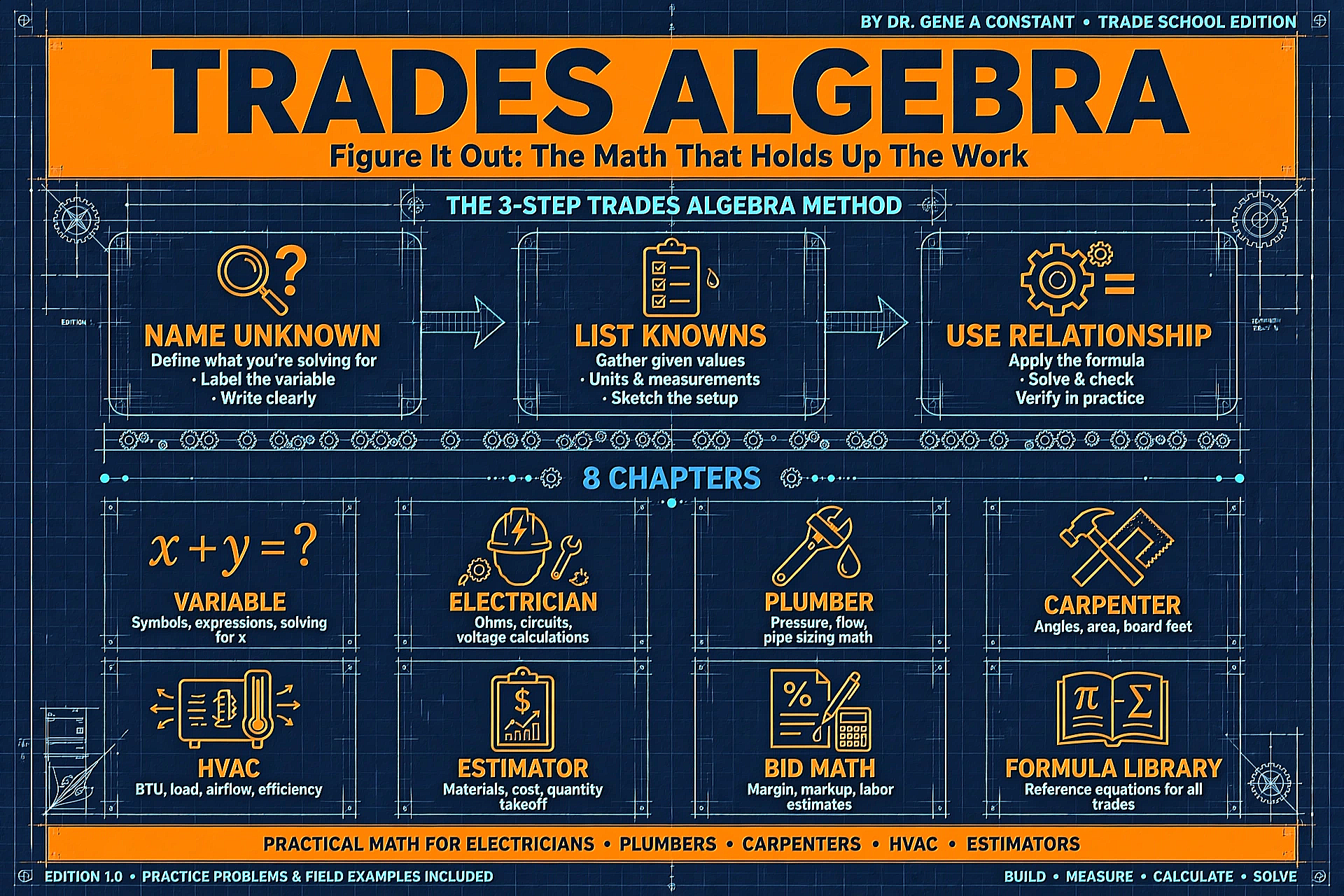
The Whole Book on One Sheet

The 3-step Trades Algebra method and all 8 chapters — the map of the territory.

↓︎ Download PNG

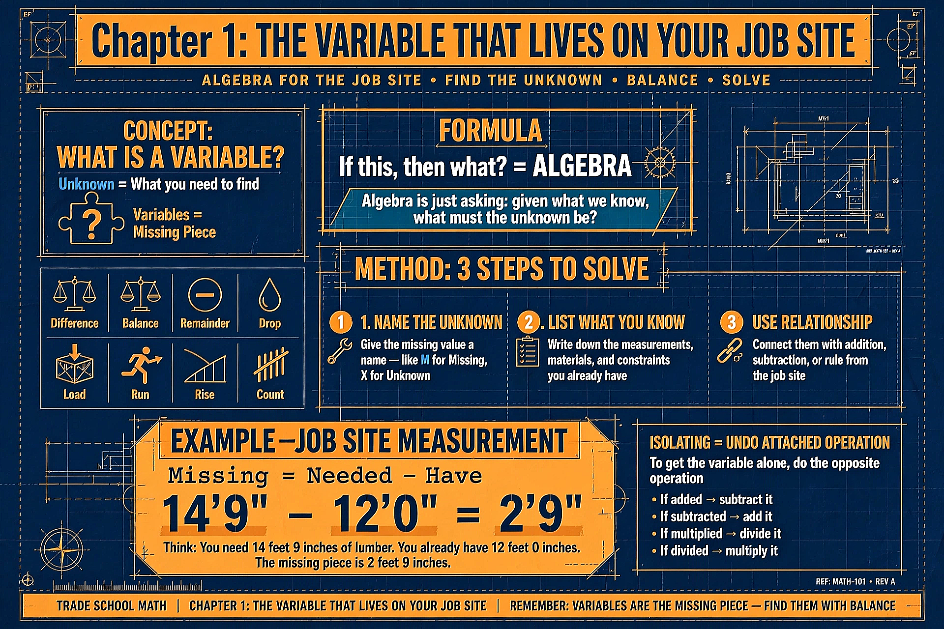
Ch. 1 — The Variable That Lives on Your Job Site

What a variable is, the 3 steps to solve, and the 14'9" job-site example.

↓︎ Download PNG

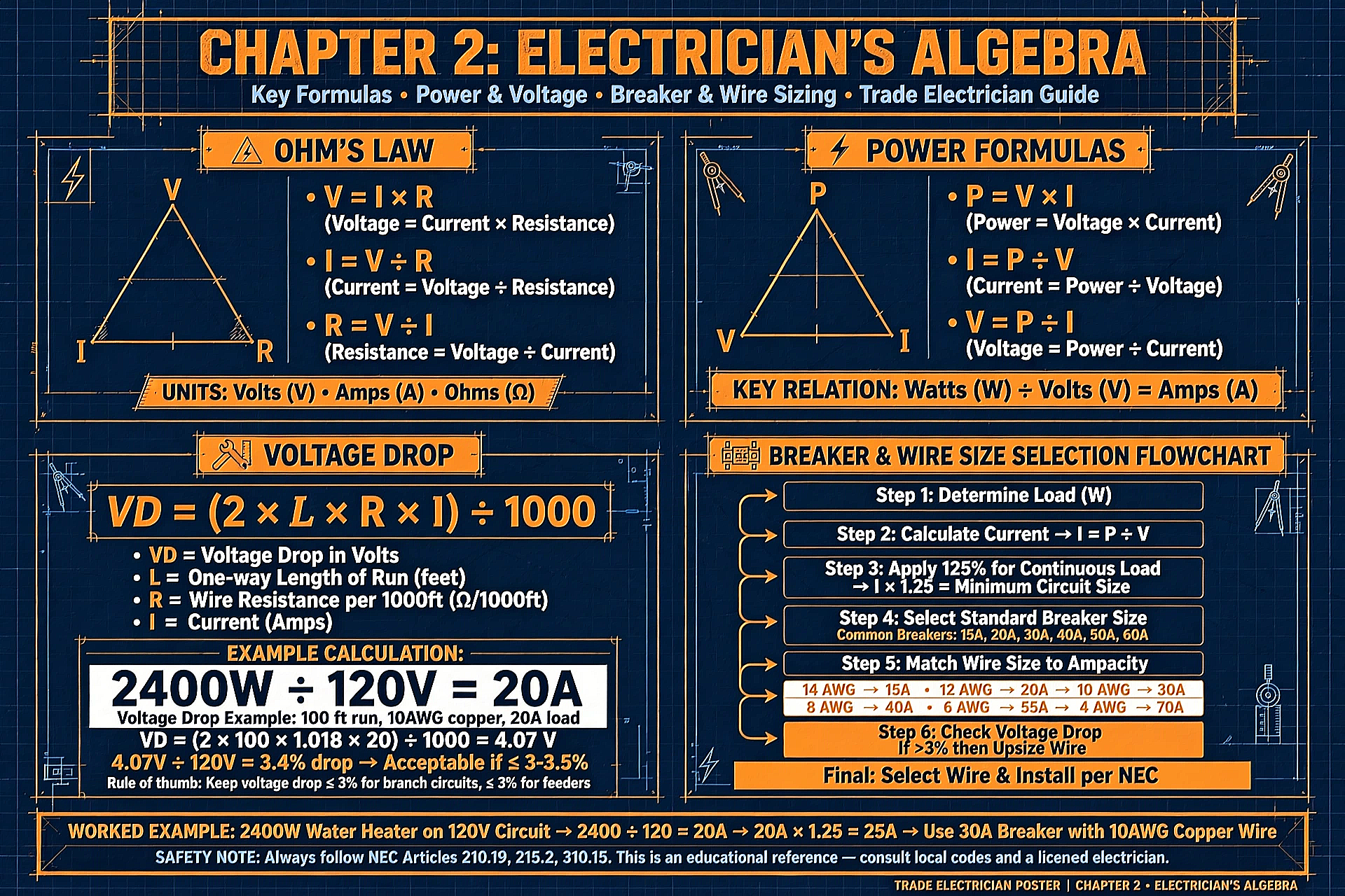
Ch. 2 — Electrician's Algebra

Ohm's Law, power formulas, voltage drop, and the breaker & wire flowchart.

↓︎ Download PNG

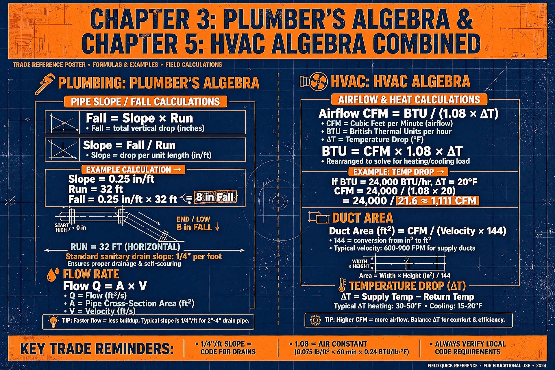
Ch. 3 & 5 — Plumber's & HVAC Algebra

Slope and fall, flow rate, airflow CFM, BTU, and duct area — combined field sheet.

↓︎ Download PNG

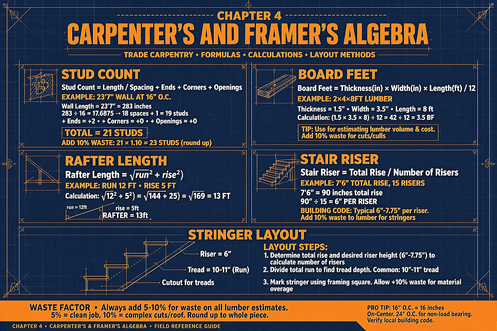
Ch. 4 — Carpenter's & Framer's Algebra

Stud count, board feet, rafter length, stair risers, and stringer layout.

↓︎ Download PNG

Ch. 6–8 — The Estimator's Handbook

Estimating, markup vs. margin, bid math, and the master cheat sheet of all trades formulas.

↓︎ Download PNG

Tax Algebra for Trades

Income flow, SE tax, payroll, markup, and the quarterly estimate — the business side.

↓︎ Download PNG

Educational reference sheets — always verify against local codes, current IRS figures, and a licensed professional for your situation.